You choose the question and judge the evidence. Laplace carries the computational work as the investigation develops.
Choose a question. Watch it unfold.01 → 03
Impact physicsRecorded session
YYouOriginal prompt
use castro to calculate asteriod collision impact with the moonuse castro to calculate asteriod collision impact with the moonuse castro to calculate asteriod collision impact with the moon
Research prompt↑
LLaplaceRecorded result
Inside the first 50 milliseconds.
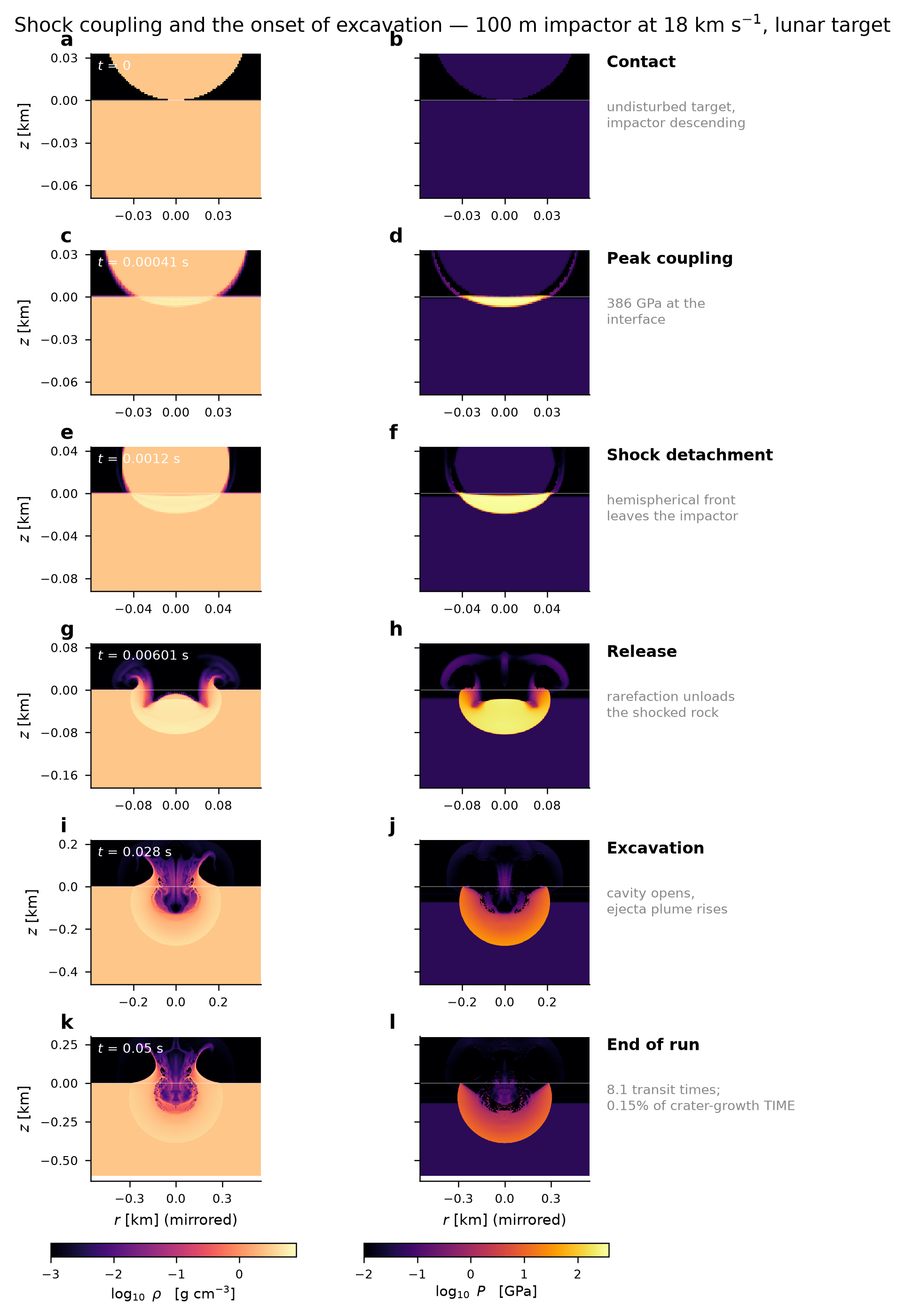
A 100 m rock strikes at 18 km/s. Explore the early shock recorded in a short lunar-impact calculation.
Original simulation movie · playback speed is illustrative
The impact simulation ends at 0.05 seconds. The final-crater estimate comes from a separate scaling law; the stellar example is an idealized toy.
Use FDS to predict a vegetation fire on sloped terrain.Use FDS to predict a vegetation fire on sloped terrain.Use FDS to predict a vegetation fire on sloped terrain.
Research prompt↑
LLaplaceRecorded result
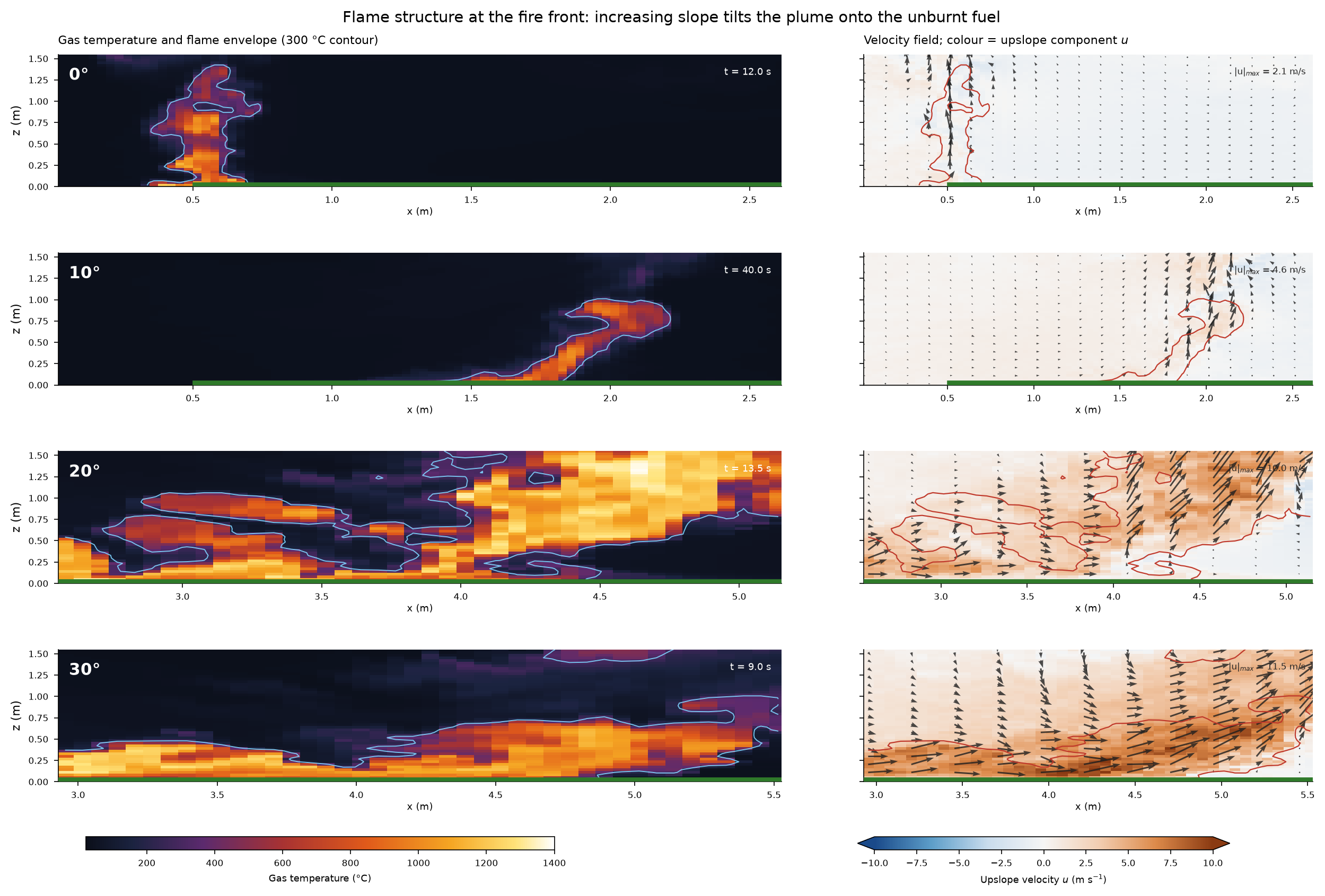
Four slopes. Watch the flame change.
Recorded FDS scenarios connect terrain, temperature, and flow. Inspect the simulated flame and the assumptions behind each comparison.
Original simulation movie · playback speed is illustrative
Reference grass fuel and no wind. Steep scenarios also use longer fuel beds and shorter ignition; slope is not isolated alone. Absolute spread rates remain unvalidated.
Develop a simple, validated computational workflow for studying HCl adsorption on generic amorphous silica: first construct several realistic hydroxylated silica surface models with different silanol arrangements and water coverages;Develop a simple, validated computational workflow for studying HCl adsorption on generic amorphous silica: first construct several realistic hydroxylated silica surface models with different silanol arrangements and water coverages;Develop a simple, validated computational workflow for studying HCl adsorption on generic amorphous silica: first construct several realistic hydroxylated silica surface models with different silanol arrangements and water coverages;
Research prompt↑
LLaplaceRecorded result
One more water molecule. A different pathway.
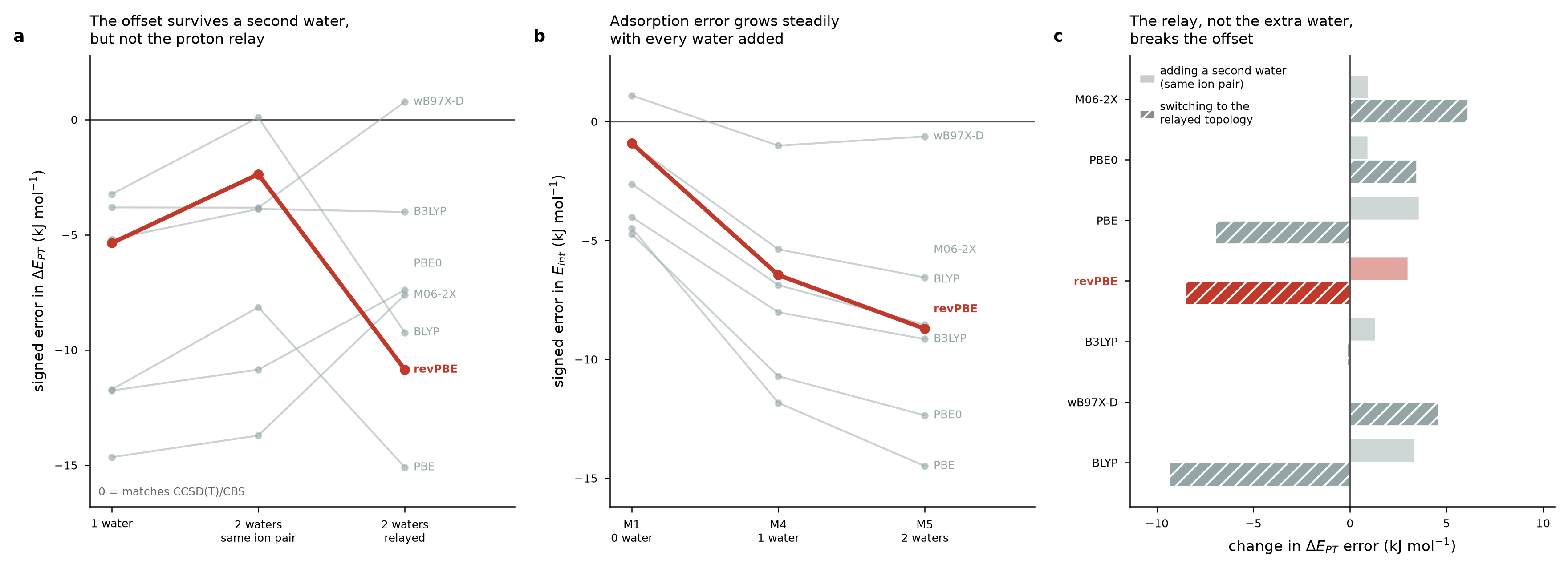
The small-cluster proton-transfer cost changed from 54.61 to 17.73 kJ/mol when a second water enabled a relay pathway.
Original study output
Small-cluster electronic energies, not measured reaction rates or a periodic-surface free-energy barrier.
Original simulation films, numerical results and model outputs, connected into one story of computational science.
An editorial film built from recorded studies. Each scene retains its model scope; playback is not live computation.
Different questions. Work you can inspect.
Move from a possibility to something you can test.
A material choice, a lighter machine, a hidden structure. See how a question becomes a model, a comparison, and a useful next step.
Aerospace engineering
Which design choices change the mass?
Explore a reduced-model search and a 65.8% lower mass-proxy solution when stage loading can vary.
Reduced-model screening, not 45 million CFD runs. The mass proxy excludes fixed per-unit overhead and requires higher-fidelity checks before a hardware decision.Inspect the design search ↗
Magnetic geophysics
What could be hiding underground?
Compare different buried models that fit the same synthetic magnetic observations over real terrain.
Synthetic magnetic observations and buried structures over real terrain. Fit ratios are not reconstruction-accuracy percentages.Explore the recovered models ↗
Particle synthesis
Which recipe should the lab try next?
Connect published recipes to particle-growth models, then examine where predictions fail to transfer.
The ammonia trend is a conditional recipe hypothesis. Held-out-publication errors of 57–178% show that transfer to a new laboratory remains unreliable.Follow the synthesis study ↗
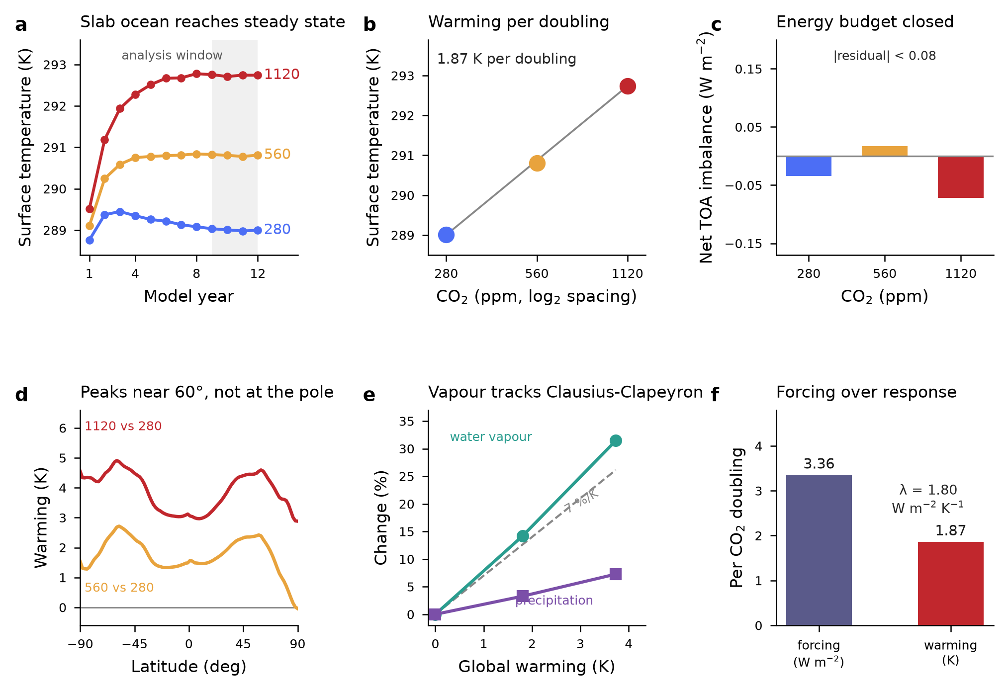
More CO₂ changes the energy balance. To see how that becomes warming, Laplace ran the same three concentrations in two model settings: first holding ocean temperature fixed, then allowing a simplified ocean to respond.
1. Select a concentration2. Switch the ocean setting3. Compare the saved results
Explore recorded results · 6 completed model runs
Turn up the CO₂. What changes?
Choose a concentration and an experiment. The display switches between the actual saved results, with the physical assumptions kept visible.
Which question are we asking?
Temperature rise relative to 280 ppm (K)
Dots are the three saved runs. The dashed connector is a visual guide; intermediate concentrations were not simulated here.
Warming vs 280 ppm+1.80 KSlab-ocean equilibrium comparison
Mean model surface temperature17.66 °CYears 9–12 of a 12-year model run
This is an idealized aquaplanet. The slab ocean is 30 m deep; there is no realistic land, sea ice, seasons or ocean circulation. These are conditional model responses, not an Earth climate-sensitivity estimate.
Direct the investigation. Inspect the work.
01
Frame the question
Set the physical problem, constraints, and the result you need to evaluate.
02
Build and run the study
Laplace prepares and executes computational work, from model inputs and code to simulations and analysis.
03
Follow the evidence
Compare alternatives, examine assumptions, and steer the next calculation.
04
Choose the next test
Identify a design worth checking, an explanation worth testing, or a measurement the model still needs.
One workspace. A growing scientific investigation.
Follow climate experiments, fluid dynamics, and geophysical inference alongside the setup and analysis needed to carry out the work. The project record keeps requests, outputs, and open questions available for inspection.
Develop a simple, validated computational workflow for studying HCl adsorption on generic amorphous silica: first construct several realistic hydroxylated silica surface models with different silanol arrangements and water coverages;Develop a simple, validated computational workflow for studying HCl adsorption on generic amorphous silica: first construct several realistic hydroxylated silica surface models with different silanol arrangements and water coverages;Develop a simple, validated computational workflow for studying HCl adsorption on generic amorphous silica: first construct several realistic hydroxylated silica surface models with different silanol arrangements and water coverages;
Research prompt↑
LLaplaceRecorded result
54.61 → 17.73 kJ/mol
Adding a second water molecule opened a proton-relay pathway in the small-cluster calculation. The comparison changed the working reaction hypothesis.
Original study output
Small-cluster electronic energies, not measured reaction rates or a periodic-surface free-energy barrier.
the design space is (1) total air flow 2ton/hr to 10ton/hr (2) altitude 50,000feet to 60,000feet (3)2bar to 4 bar (4)mach 0.7 to 0.9; optimizioan should be on total mass and/or fuel; no need to cool the pressurzied air generated; add some 3D visualziation, the report should read as an optimization report that generate and explain what is the best systemthe design space is (1) total air flow 2ton/hr to 10ton/hr (2) altitude 50,000feet to 60,000feet (3)2bar to 4 bar (4)mach 0.7 to 0.9; optimizioan should be on total mass and/or fuel; no need to cool the pressurzied air generated; add some 3D visualziation, the report should read as an optimization report that generate and explain what is the best systemthe design space is (1) total air flow 2ton/hr to 10ton/hr (2) altitude 50,000feet to 60,000feet (3)2bar to 4 bar (4)mach 0.7 to 0.9; optimizioan should be on total mass and/or fuel; no need to cool the pressurzied air generated; add some 3D visualziation, the report should read as an optimization report that generate and explain what is the best system
Research prompt↑
LLaplaceRecorded result
65.8% lower modelled mass proxy.
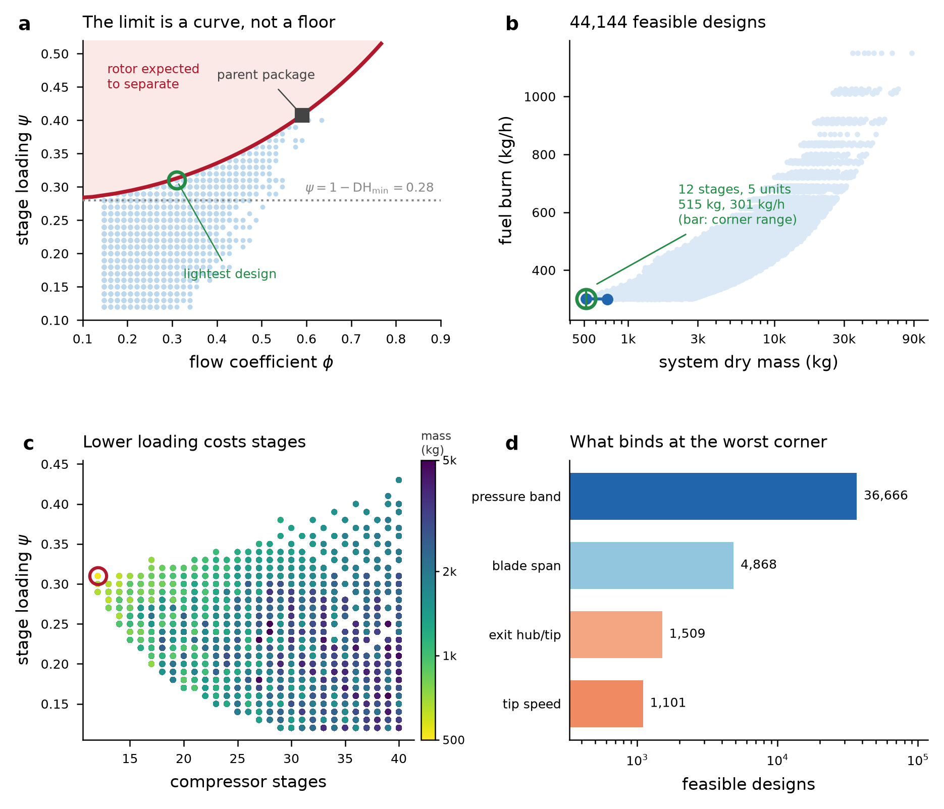
A reduced-model search screened 45.16 million candidate grid points. Variable stage loading reached 515.2 kg versus 1,505.5 kg with fixed loading.
Original study output
Reduced-model screening, not 45 million CFD runs. The mass proxy excludes fixed per-unit overhead and requires higher-fidelity checks before a hardware decision.
can you think of a quick an simple simulation that demonstrate climate change by increasing CO2? need to be very computation light onecan you think of a quick an simple simulation that demonstrate climate change by increasing CO2? need to be very computation light onecan you think of a quick an simple simulation that demonstrate climate change by increasing CO2? need to be very computation light one
Research prompt↑
LLaplaceRecorded result
Six experiments. Two distinct responses.
At 280, 560, and 1,120 ppm, fixed-temperature runs isolate energy forcing while slab-ocean runs allow warming. Explore the six saved scenarios in the full study.
Original study output
Idealized aquaplanet with a 30 m slab ocean, without realistic land, sea ice, seasons, or ocean circulation. These responses are not an Earth climate-sensitivity estimate.
Use FDS to predict a vegetation fire on sloped terrain.Use FDS to predict a vegetation fire on sloped terrain.Use FDS to predict a vegetation fire on sloped terrain.
Research prompt↑
LLaplaceRecorded result
Four slopes. Temperature and flow made visible.
FDS runs at 0°, 10°, 20°, and 30° produced fields, diagnostics, and comparison movies to investigate how terrain changes the fire.
Original study output
Reference grass fuel and no wind. Steep scenarios also use longer fuel beds and shorter ignition; slope is not isolated alone. Absolute spread rates remain unvalidated.
create a 3D simulation of that; with real earth datacreate a 3D simulation of that; with real earth datacreate a 3D simulation of that; with real earth data
Research prompt↑
LLaplaceRecorded result
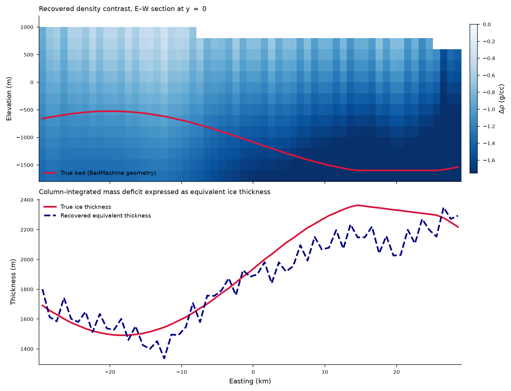
Two underground models fit the signal.
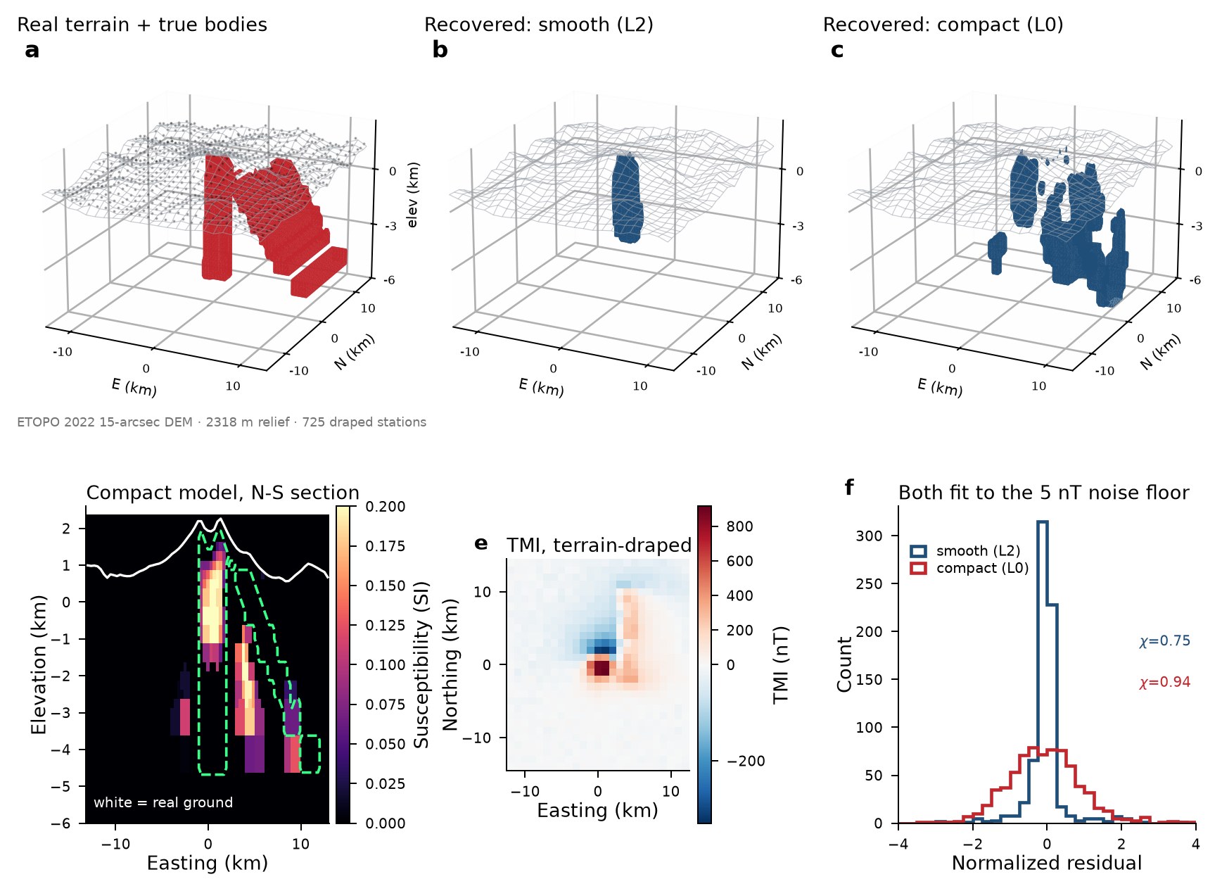
A 725-station synthetic magnetic survey over real terrain supported different recovered models. The comparison made non-uniqueness visible.
Original study output
Synthetic magnetic observations and buried structures over real terrain. Fit ratios are not reconstruction-accuracy percentages.
assume silica coated with TMMS, estimate its contact angle with water from first prinicipple (without quoting observation); start with analytical modelassume silica coated with TMMS, estimate its contact angle with water from first prinicipple (without quoting observation); start with analytical modelassume silica coated with TMMS, estimate its contact angle with water from first prinicipple (without quoting observation); start with analytical model
Research prompt↑
LLaplaceRecorded result
A texture hypothesis to test.
The analytical coating model gave 115.3°. After the user supplied a 130° measurement, the study examined how particle packing could explain the gap.
Original study output
Analytical and geometric models. The 130° measurement was disclosed before the texture explanation; this was not a blind prediction.
Create a reproducible simulation of Stöber silica nanosphere synthesis using open-source software.

Use:
- Cantera for TEOS hydrolysis and condensation kinetics
- OpenFOAM’s population-balance model for nucleation, particle growth, and aggregation
- Python with SciPy, pandas, and matplotlib forCreate a reproducible simulation of Stöber silica nanosphere synthesis using open-source software.
Use:
- Cantera for TEOS hydrolysis and condensation kinetics
- OpenFOAM’s population-balance model for nucleation, particle growth, and aggregation
- Python with SciPy, pandas, and matplotlib forCreate a reproducible simulation of Stöber silica nanosphere synthesis using open-source software.
Use:
- Cantera for TEOS hydrolysis and condensation kinetics
- OpenFOAM’s population-balance model for nucleation, particle growth, and aggregation
- Python with SciPy, pandas, and matplotlib for
Research prompt↑
LLaplaceRecorded result
A recipe hypothesis, with a transfer gap.
The study assembled 209 published measurement rows and connected kinetics to particle growth. Held-out-publication errors of 57–178% exposed the need for local calibration.
Original study output
The ammonia trend is a conditional recipe hypothesis. Held-out-publication errors of 57–178% show that transfer to a new laboratory remains unreliable.
use castro to calculate asteriod collision impact with the moonuse castro to calculate asteriod collision impact with the moonuse castro to calculate asteriod collision impact with the moon
Research prompt↑
LLaplaceRecorded result
The first 50 milliseconds of impact.
The lunar-impact chapter recorded a peak pressure of about 385.7 GPa, compared with a 391.4 GPa analytic reference. Earlier chapters explored fluid instability and a stellar-layer toy.
Original study output
The impact simulation ends at 0.05 seconds. The final-crater estimate comes from a separate scaling law; the stellar example is an idealized toy.
Run a small CESM real-physics smoke test, from case setup through completed output.Run a small CESM real-physics smoke test, from case setup through completed output.Run a small CESM real-physics smoke test, from case setup through completed output.
Research prompt↑
LLaplaceRecorded result
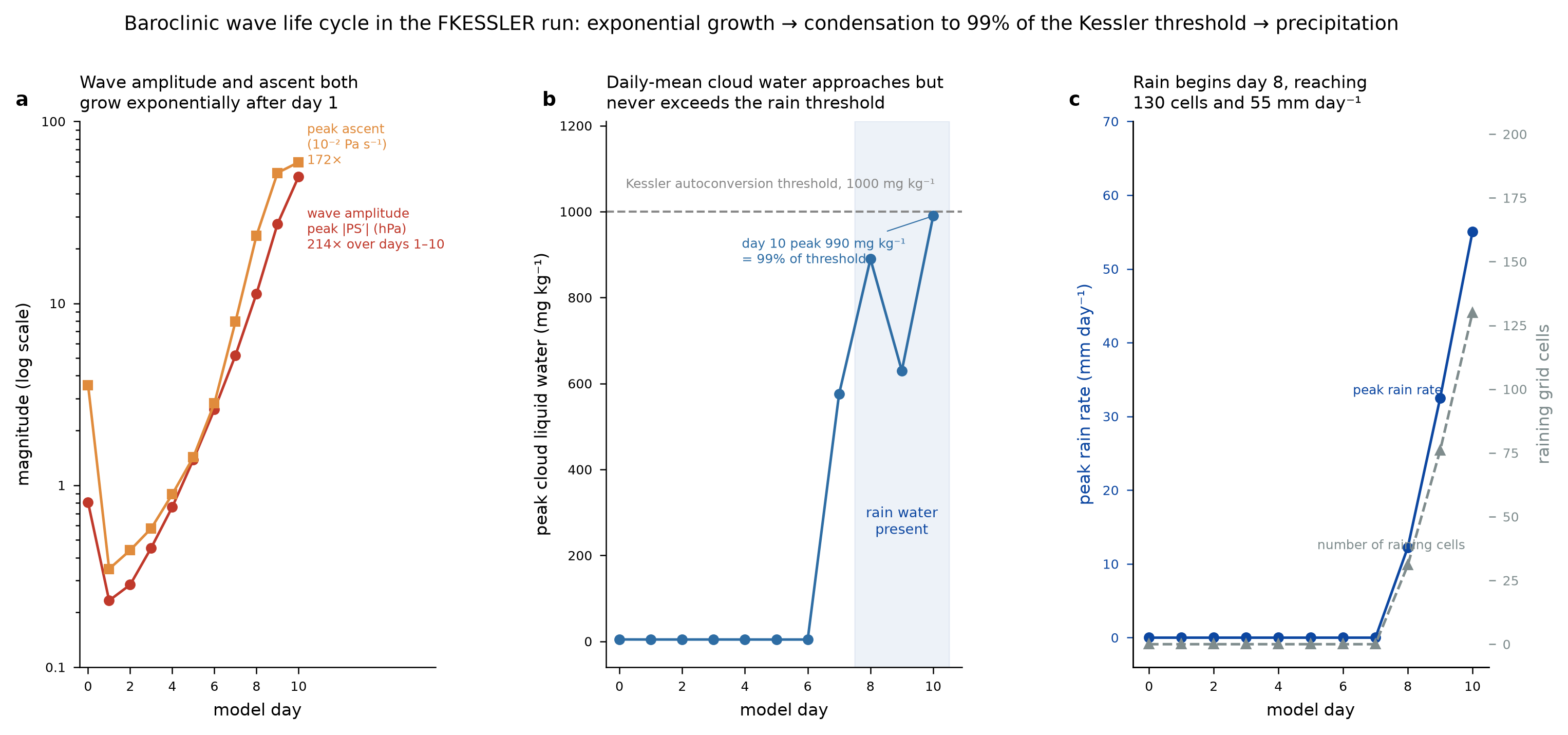
Ten days of growing weather patterns.
Expanded from the initial one-day request, the investigation produced a ten-day atmospheric-wave study, diagnostic tables, a globe artifact, and explanatory movies.
Original study output
Idealized model dynamics. The 214× figure measures pressure-wave growth, not computational speed or forecast accuracy.
Run a very simple CESM simulation, should be 1 month, think about the simplest quickest way to see some interesting physicsRun a very simple CESM simulation, should be 1 month, think about the simplest quickest way to see some interesting physicsRun a very simple CESM simulation, should be 1 month, think about the simplest quickest way to see some interesting physics
Research prompt↑
LLaplaceRecorded result
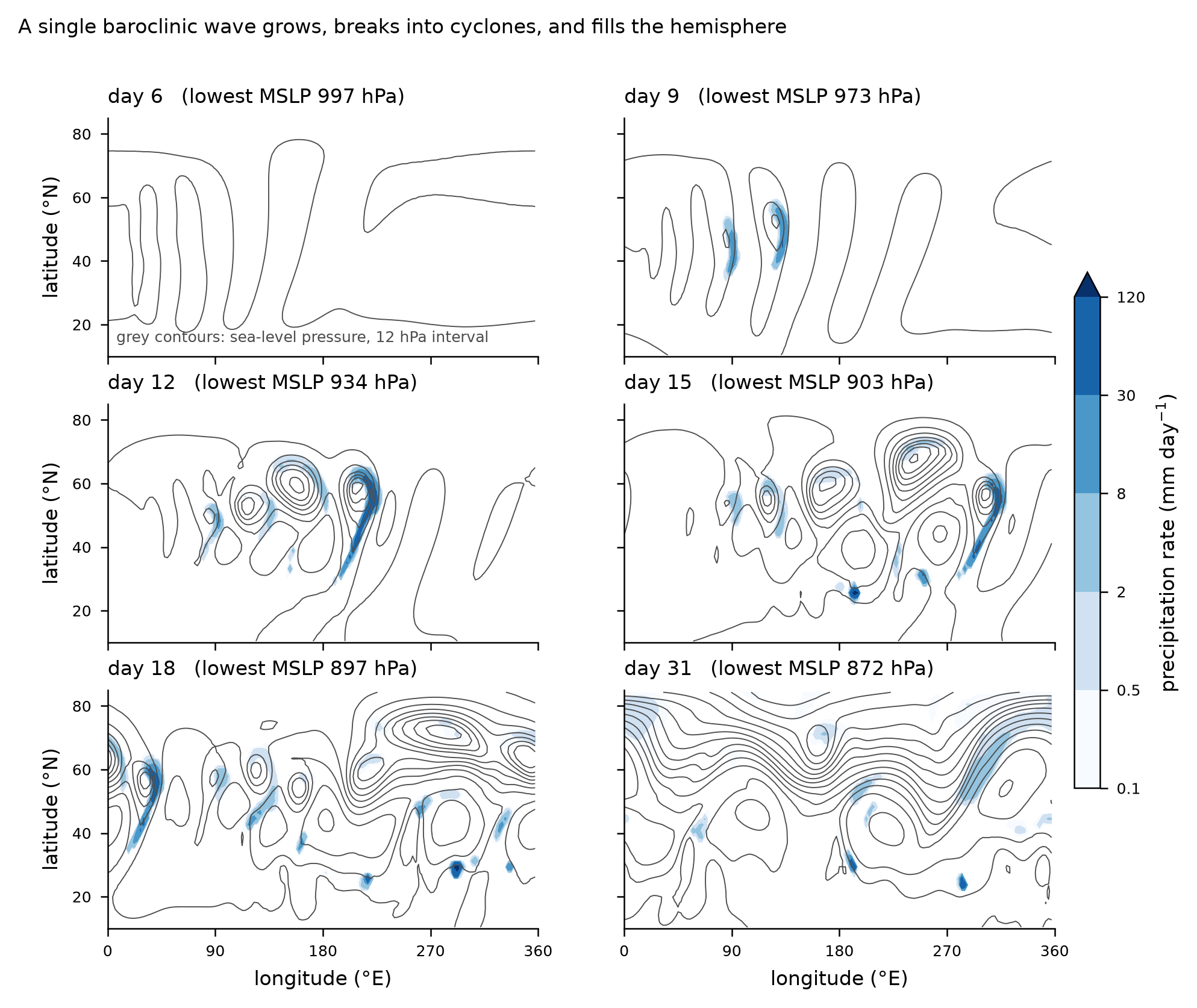
31 model days, ready to inspect.
The recorded study produced 249 diagnostic samples at three-hour intervals, two charts, and an explanatory movie connecting the evolution of the atmosphere to its underlying dynamics.
Original study output
Simulated duration, not elapsed work. The original lifecycle figure retains a stale pressure label; this is not a real-world forecast.
create a sample WRF weather simulationcreate a sample WRF weather simulationcreate a sample WRF weather simulation
Research prompt↑
LLaplaceRecorded result
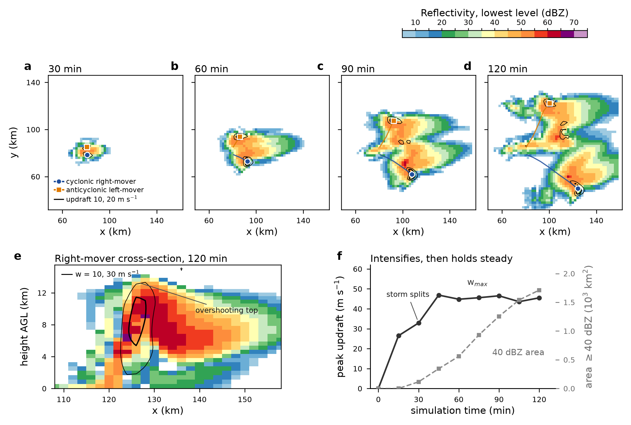
A simulated storm. A simpler explanation to compare.
Two simulated hours in WRF became a storm-splitting investigation, followed by a reduced physical model and a paper comparing selected diagnostics.
Original study output
One idealized WRF atmosphere, not a real-world forecast. Agreement varies by diagnostic; the source paper retains rainfall-window and vorticity-caption inconsistencies.
create a model for fludiztion of silica 500 nm spheres powder; search for relevant open source programcreate a model for fludiztion of silica 500 nm spheres powder; search for relevant open source programcreate a model for fludiztion of silica 500 nm spheres powder; search for relevant open source program
Research prompt↑
LLaplaceRecorded result
Clumps, vibration, and the next experiment.
A 1,600-clump particle study explored vibration. A separate analytical model estimated a conditional gas-velocity range; the particle runs themselves contained no gas.
Original study output
The particle runs contain no gas and their initial packing was still settling. Clump size is calibrated; this is not a validated fluidized-bed operating point.
use SemPeg, think about some kind of data you get from your earthdata API, and apply a 3D simulation by SImPeg trying to understand and explain the datause SemPeg, think about some kind of data you get from your earthdata API, and apply a 3D simulation by SImPeg trying to understand and explain the datause SemPeg, think about some kind of data you get from your earthdata API, and apply a 3D simulation by SImPeg trying to understand and explain the data
Research prompt↑
LLaplaceRecorded result
A close data fit, with depth still unresolved.
When real-data acquisition failed, the study used a synthetic gravity example. A near-target misfit and mass recovery did not establish reliable depth recovery.
Original study output
Synthetic substitute after real-data acquisition failed. The original figure retains a misleading BedMachine label; depth recovery remains unresolved.
Run a minimal CESM infrastructure test: compset X with dead model components, resolution f19_g17, and a one-day run. Create the case, build it, submit it, confirm time-stepping and summarize the output.Run a minimal CESM infrastructure test: compset X with dead model components, resolution f19_g17, and a one-day run. Create the case, build it, submit it, confirm time-stepping and summarize the output.Run a minimal CESM infrastructure test: compset X with dead model components, resolution f19_g17, and a one-day run. Create the case, build it, submit it, confirm time-stepping and summarize the output.
Research prompt↑
LLaplaceRecorded result
A completed build-to-output check.
The record reports a one-model-day smoke test, a 35-second model execution, and restart output. This established an infrastructure receipt for subsequent work.
▤cesm_smoke_test_report.mdSaved
Infrastructure smoke test with dead model components. No climate finding is claimed.
Help me create a new specialist: a Manim visualization skill.Help me create a new specialist: a Manim visualization skill.Help me create a new specialist: a Manim visualization skill.
Research prompt↑
LLaplaceRecorded result
A rendering workflow with a working example.
The session configured a visualization specialist and supplied a Manim test scene and its rendered MP4.
▤Manim scene sourceSaved
▤Rendered test movieSaved
A visualization setup and render check, not a new physical simulation.
what is the compute power modal.com use?what is the compute power modal.com use?what is the compute power modal.com use?
Research prompt↑
LLaplaceRecorded result
A compute research note.
The conversation compares scientific-cluster and elastic-cloud hardware. It provides historical research context; no matched performance experiment was run.
▤Conversation and source referencesSaved
No simulation or matched performance benchmark. Historical hardware and pricing claims are not current buying advice.
use openfoam to do a RANS turbulence modeling of supersonic gas eductoruse openfoam to do a RANS turbulence modeling of supersonic gas eductoruse openfoam to do a RANS turbulence modeling of supersonic gas eductor
Research prompt↑
LLaplaceRecorded result
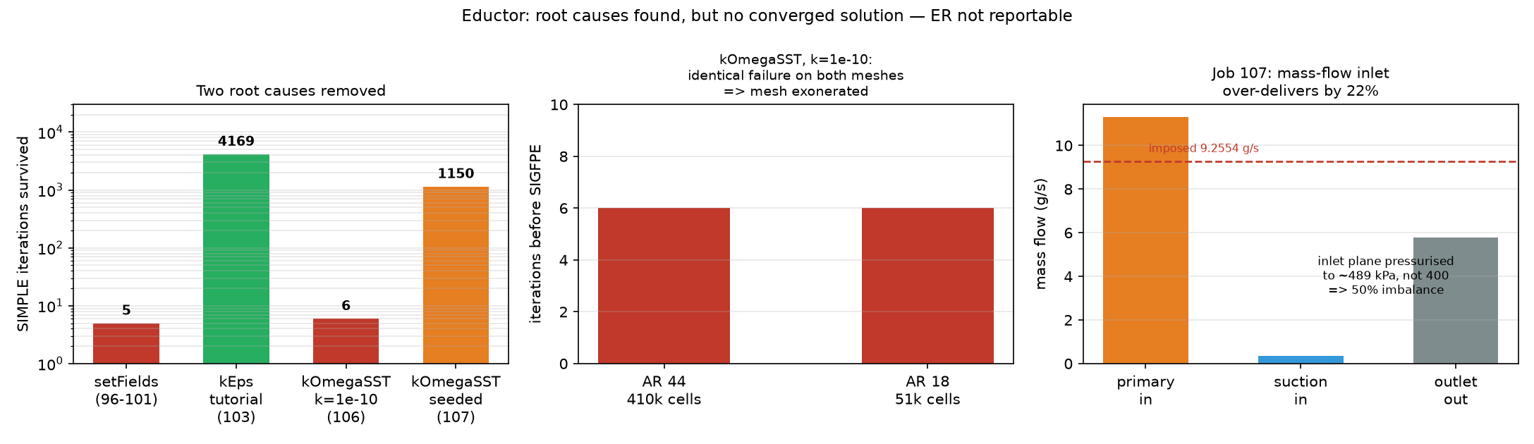
A diagnosis, with performance unresolved.
The staged CFD case reached 410,400 cells, but mass imbalance remained around 50%. The useful output was the failure diagnosis and a proposed next solver test.
Original study output
No accepted entrainment ratio. A transient-solver alternative was proposed but not run successfully in this record.
One workspace. A growing scientific investigation.
Follow climate experiments, fluid dynamics, and geophysical inference alongside the setup and analysis needed to carry out the work. The project record keeps requests, outputs, and open questions available for inspection.
↺ Run → inspect → revise, with researcher steering
HUMANReview + decide
Technical execution delegatedModels, runs, and processing are carried through the investigation.
Comparisons assembledScenario results and analysis are presented together.
Evidence stays connectedInspect the inputs, outputs, revisions, and next test.
Illustrates work ownership. Box widths are schematic; human time saved was not measured.
Ask the next question.
The scientific work develops as the question changes. Add a molecular assumption, widen a design search, or compare a different model configuration. The demonstrations show how requests, calculations, and revisions accumulate in a working investigation.
Make computational scale available through conversation.
An R&D team should be able to explore more models, more conditions and more design choices without rebuilding its workflow for every question.
Laplace connects scientific modelling, code execution, simulation, and analysis around the researcher’s question. The studies demonstrate work across molecular chemistry, engineering design, climate, and other physical systems, with evidence kept alongside the work as it develops.
The unit of work is an investigation.
A useful scientific result depends on model choices, execution, comparison, and interpretation. Laplace carries work across those steps while researchers direct the question and evaluate the evidence.
A record that develops with the question.
Prompts, code, inputs, outputs, and corrections remain connected to their studies. Explore the project to see what accumulated across related investigations.
From capability to repeatable value.
The next proof is value on a defined customer workflow, measured through accepted results, expert effort, human interventions, and compute cost. These demonstrations establish computational work; they do not yet measure that commercial outcome.
Here, Laplace configures and executes scientific tools. The examples do not establish a trained solver-replacement model or a general speed advantage.
Why does water bead more strongly than the chemistry predicts?
The prompt → the result
Surface physicsRecorded session
YYouOriginal prompt
assume silica coated with TMMS, estimate its contact angle with water from first prinicipple (without quoting observation); start with analytical modelassume silica coated with TMMS, estimate its contact angle with water from first prinicipple (without quoting observation); start with analytical modelassume silica coated with TMMS, estimate its contact angle with water from first prinicipple (without quoting observation); start with analytical model
Research prompt↑
LLaplaceRecorded result
A texture hypothesis to test.
The analytical coating model gave 115.3°. After the user supplied a 130° measurement, the study examined how particle packing could explain the gap.
Analytical and geometric models. The 130° measurement was disclosed before the texture explanation; this was not a blind prediction.
The result summarizes the recorded session, including later requests and review.
Read the research prompt
Original research prompt
assume silica coated with TMMS, estimate its contact angle with water from first prinicipple (without quoting observation); start with analytical model
One calculation connects molecular packing to a visible surface property, then tests how the result changes with coverage.
Analytical calculations and sensitivity tests. The observed contact angle was known before the texture explanation was proposed.
Surface texture could explain the extra water repellency.
A water droplet can reveal a mismatch between a material’s chemistry and the structure of its surface. Laplace built a coating model, found a lower intrinsic contact angle, and examined particle packing as a possible explanation for the observed beading. The investigation identified an experiment to distinguish chemistry from texture.
Study scope. Analytical and geometric models. The 130° measurement was disclosed before the texture explanation; this was not a blind prediction.
Inspect the result evidence and download the outputs
Computed baseline: 115.3° intrinsic contact angle under the model’s baseline assumptions. Evidence ↗
Explanation to test: 125–129° for the considered sphere packings, assuming a suspended drop. Evidence summary ↗
Usable handoff: Original calculation code, result files and a proposed hysteresis/packing test. Evidence ↗
The measured 130° was disclosed before the texture explanation was developed. The wetting state remains unconfirmed, and the intrinsic angle has substantial parameter uncertainty.
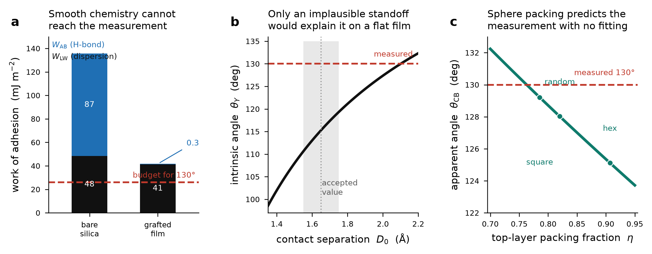
The produced figure: chemistry, sensitivity and sphere packing. Saved output from this investigation; no new calculation runs in this page.
Model and method
Yes, this includes simulation. Laplace numerically builds and packs molecular groups on a model surface, tests water access, and combines those results with an interfacial-energy calculation. The configurations are static; this is not an atom-by-atom molecular-dynamics trajectory.
How the investigation developed.
An engineer wants to know how water should wet silica coated with trimethylsilyl groups. A contact angle describes how much a drop beads up: a larger angle means less spreading. A single answer matters less than knowing which physical lever controls it. Should the team change the coating chemistry, remove more hydroxyl groups, or change how the particles are deposited?
01
Start from chemistry rather than fitting the angle
The initial request was to estimate the angle from first principles, starting analytically. Laplace assembled a dispersion-force model, built a geometric coating, and estimated which leftover hydroxyl groups a water molecule could reach. The early report gave about 116°; the final refined baseline is 115.3°. It used known material properties and an empirical contact-separation parameter, without using an input contact-angle measurement. The exact final baseline should not be read as a timestamped prediction made before every later revision.
02
Find the mechanism hidden by a surface-chemistry count
The model leaves about 39% of hydroxyl sites unreacted because the coating groups physically crowd one another. What matters is accessibility: the coating shelters the remaining sites. In the model, making those sites accessible would lower the angle to 87.8°. That gives the team a concrete hypothesis: changing the chemical count alone may miss what water actually encounters.
03
Use a discrepancy to change the question
The user then disclosed a measured angle of 130°. Laplace examined a textured bed of silica spheres rather than forcing the smooth-surface model to fit. Assuming water is suspended on the sphere tops, the model gives 125.1–129.2° across the considered packings. The useful output is an explanation to test: particle packing and trapped air may account for the difference between the chemistry and the measurement.
The chemistry-to-texture explanationOriginal result
Original final-session figure. Left: the adhesion budget. Middle: the contact-separation sensitivity. Right: packing changes the apparent angle. Read the 125–129° range as conditional on the suspended-drop model, and alongside the report's wider intrinsic-angle uncertainty. reconciliation.png · Evidence summary ↗
The next test
Test the proposed wetting state before changing the chemistry. Advancing/receding contact angles or a tilt test can probe pinning and hysteresis; microscopy can constrain the packing fraction. These are proposed experiments, not completed validation.
Scientific assumptions and limitations
The assumed contact separation is a major uncertainty: the report gives a 98.6–125.9° intrinsic-angle range over its wider parameter interval. The baseline 115.3° is not a high-precision accuracy claim.
The 130° measurement was disclosed before the textured-surface explanation was developed. Agreement is post-disclosure consistency, not independent predictive validation.
The suspended wetting state and sample packing were not directly observed. Static geometry omits thermal motion and does not predict hysteresis.
The same questionWhy does coated silica bead water, and why does the sample read 130°?
Direct the investigation. Inspect the work.
Laplace carries technical execution while researchers set the question, steer the study, and evaluate the evidence.
A team-managed workflowIllustrative workflow with existing tools
Task 1Define the surface
→
Task 2Build the physical model
→
Task 3Implement and run
→
Task 4Check the discrepancy
→
Task 5Assemble the handoff
The team coordinates tools, context, and revisions across the study.
With LaplaceTechnical work demonstrated in these studies
HUMANBrief + steer
Laplace carries the technical work
Frame chemistry and packingConnect physics in codeRun scenariosChallenge the explanationDeliver an inspectable study
↺ Run → inspect → revise, with researcher steering
HUMANReview + decide
Task execution delegatedModel setup, code and output processing are carried inside the recorded investigation.
Revisions stay connectedChanges to the brief and diagnostic corrections share a working record.
Results arrive togetherInspect the files, findings and next test in one handoff.
Illustrates work ownership. Box widths are schematic; human time saved was not measured.
Inspect the work inside the Laplace block
Frame chemistry and packing. Build the molecular layer and its water-accessibility test.
Connect physics in code. Combine dispersion, hydrogen bonding and a wetting relation.
Run scenarios. Explore residual sites, calcination, corrugation and sphere packing.
Challenge the explanation. Investigate the disclosed 130° angle; check sensitivities and claims.
Deliver an inspectable study. Save code, numeric results, figures and a falsifiable mechanism.
↺Both routes need iteration when the model and measurement disagree.
The same physical tasks are connected inside a model–run–review workflow. The useful gain to test is less manual assembly and a faster route to the next experiment.
What this study gathered.
Evidence gathered
A reusable physics calculation
Original code, results JSON, adhesion checks and the final report.
A conventional investigation would connect several pieces of work: surface chemistry and coverage assumptions, a model of how coating molecules fit, interfacial-force calculations, a wetting model, and a comparison with the actual sample. An empirical fit could match an observed angle while hiding the mechanism. A detailed molecular-dynamics study would instead require an appropriate force model and its own sampling and validation effort. Neither route's human effort or total elapsed time was measured in this session.
How to read the timing
These investigations often continued across separate visits. The first and last messages do not measure continuous work.
4d 22h 40m 15sCalendar span of the conversation
50mCombined child-agent windows, with overlapping intervals counted once
Agent windows can include waiting and omit work in the main conversation. They are not a measure of active human work, total compute or time saved. The exports do not provide a reliable labour clock.
Develop a simple, validated computational workflow for studying HCl adsorption on generic amorphous silica: first construct several realistic hydroxylated silica surface models with different silanol arrangements and water coverages;Develop a simple, validated computational workflow for studying HCl adsorption on generic amorphous silica: first construct several realistic hydroxylated silica surface models with different silanol arrangements and water coverages;Develop a simple, validated computational workflow for studying HCl adsorption on generic amorphous silica: first construct several realistic hydroxylated silica surface models with different silanol arrangements and water coverages;
Research prompt↑
LLaplaceRecorded result
54.61 → 17.73 kJ/mol
Adding a second water molecule opened a proton-relay pathway in the small-cluster calculation. The comparison changed the working reaction hypothesis.
Small-cluster electronic energies, not measured reaction rates or a periodic-surface free-energy barrier.
The result summarizes the recorded session, including later requests and review.
Read the research prompt
Selected research prompt excerpt
Develop a simple, validated computational workflow for studying HCl adsorption on generic amorphous silica: first construct several realistic hydroxylated silica surface models with different silanol arrangements and water coverages;
Four calculations at a time turn a numerical-settings question into a 52-point convergence study.
About 60 minutes for one later CP2K convergence batch, reported across two jobs. This does not time the entire chemistry study or its separate molecular-dynamics demonstration.
One added water molecule changes the reaction hypothesis.
Water near a silica surface can change how an acid reacts. Laplace compared molecular clusters with one and two water molecules. The second water provided a proton-relay pathway, helping a hydrogen ion move between sites and lowering the computed transfer cost from 54.61 to 17.73 kJ/mol. That comparison changed the working reaction hypothesis and pointed to the surface calculations and measurements needed next.
Study scope. Small-cluster electronic energies, not measured reaction rates or a periodic-surface free-energy barrier.
Inspect the result evidence and download the outputs
Computed mechanism change: One versus two waters changed the cluster electronic proton-transfer cost from 54.61 to 17.73 kJ/mol. Evidence ↗
Executed demonstration: 120 ps of sampling on a 14-atom GFN2-xTB cluster, with numerical diagnostics. Evidence summary ↗
Usable handoff: Quantum benchmarks, method comparisons, inputs, sampling diagnostics and next research steps. Evidence summary ↗
No periodic adsorption-energy result or production periodic molecular dynamics was completed. The nitric-acid extension produced a pipeline and structures, not composite nitric-acid energetics.
54.61 → 17.73Computed proton-transfer cost, kJ/molOne-water versus two-water cluster electronic energies. These are not measured reaction rates or a periodic free-energy barrier.Evidence summary ↗
120 psDemonstration samplingSix 20-ps walkers on a 14-atom GFN2-xTB cluster; simulated physical time, not elapsed runtime.Evidence summary ↗
The produced figure: how the water-assisted pathway changes method error. Saved output from this investigation; no new calculation runs in this page.
Model and method
Yes. This session contains actual quantum-chemistry calculations and 120 ps of enhanced-sampling molecular dynamics on a small cluster using GFN2-xTB. It also contains periodic CP2K convergence probes. A completed periodic adsorption study or production ab-initio molecular-dynamics campaign is not established.
How the investigation developed.
How does hydrogen chloride land on, react with, and leave a silica surface? The answer changes with the surface's hydroxyl sites and its water coverage. An R&D team needs to know which assumptions dominate the result and which measurement would reduce uncertainty, rather than receiving a single rate for an unspecified surface.
01
Make the workflow executable
Laplace built a connected workflow with surface models, quantum benchmarks, a comparison of seven density-functional methods, simulation inputs, enhanced sampling, and a kinetics module. On initially limited hardware, it ran what was tractable and specified larger calculations separately. The 120-ps dynamics demonstration checked the sampling machinery on a small cluster; it did not simulate an extended silica surface at production fidelity.
02
Extend the calculation where the assumption matters
After cluster access became available, Laplace added missing molecular models and tested numerical settings. The important scientific result came from a second water molecule: the computed proton-transfer cost fell from 54.61 to 17.73 kJ/mol. A controlled comparison separated ordinary solvation from a proton-relay pathway. Water was participating in the mechanism, rather than merely changing the environment.
03
Let better evidence overturn the earlier story
The extension exposed limits in the first-stage picture. A functional-error correction changed on the relay geometry. The proposed plane-wave cutoff failed the project's force criterion. Repairing defective surface structures collapsed the intended hydroxyl-density ladder, prompting a different construction method. The output therefore includes revised models and an explicit account of which earlier claims no longer survive.
The pathway changes the method's errorOriginal result
Original session figure. The comparison distinguishes adding water from enabling a proton relay. It shows why one blanket computational correction can fail on a different reaction geometry. functional_error_1w_vs_2w.png · Evidence summary ↗
A real simulation, with a defined level of fidelityOriginal result
Original demonstration output: free-energy surfaces and sampling diagnostics for the small GFN2-xTB cluster. The apparent agreement with a higher-level energy is explicitly called coincidental in the report. Desorption was not converged; this is not a quantitative prediction for the periodic surface. fes_demo.png · Evidence summary ↗
Detect a broken model set, then rebuild itOriginal result
Original session figure. Repairing defects changed the hydroxyl density; an alternative construction recovered a usable ladder over a narrower range. The lowest originally intended densities remain unrepresented. ladder_rebuilt.png · Evidence summary ↗
The next test
Compute relaxed periodic adsorption energies on the rebuilt surfaces, then compare uptake against independently measured water coverage and site populations. The session narrows the next research step; it does not close the full material-validation problem.
Scientific assumptions and limitations
The headline 54.61→17.73 kJ/mol compares cluster electronic-energy costs. It should not be described as a measured acceleration or a converged periodic free-energy barrier.
The 52 periodic calculations were numerical convergence probes on unrelaxed geometries. No periodic adsorption energy or full periodic ab-initio dynamics result was produced.
The updated hydration curve and topology-dependent error were not propagated through the full original uncertainty calculation. Experimental comparison remains prospective.
The HNO3 extension delivered a generalised pipeline and structures, but no composite HNO3 energetics. Some first-stage limitation prose remains stale; the later methods, second-stage results and numeric files determine this case study's scope.
The same questionWhich surface and water assumptions control HCl reaction predictions?
Direct the investigation. Inspect the work.
Laplace carries technical execution while researchers set the question, steer the study, and evaluate the evidence.
A team-managed workflowIllustrative workflow with existing tools
Task 1Build surface and cluster models
→
Task 2Choose and benchmark methods
→
Task 3Prepare compute and sampling
→
Task 4Connect chemistry to rates
→
Task 5Review and plan validation
The team coordinates tools, context, and revisions across the study.
With LaplaceTechnical work demonstrated in these studies
HUMANBrief + steer
Laplace carries the technical work
Generate the model setRun quantum benchmarksExecute at stated fidelityRevise the mechanismPackage the next research step
↺ Run → inspect → revise, with researcher steering
HUMANReview + decide
Task execution delegatedModel setup, code and output processing are carried inside the recorded investigation.
Revisions stay connectedChanges to the brief and diagnostic corrections share a working record.
Results arrive togetherInspect the files, findings and next test in one handoff.
Illustrates work ownership. Box widths are schematic; human time saved was not measured.
Inspect the work inside the Laplace block
Generate the model set. Construct surface/cluster assets and record their assumptions.
Run quantum benchmarks. Compare seven functionals and extend to the second-water models.
Execute at stated fidelity. Run 120 ps of cluster sampling and periodic convergence probes.
Revise the mechanism. Separate solvation from proton relay; identify failed numerical criteria.
Package the next research step. Deliver artifacts, corrected scope and a periodic/experimental plan.
↺Review sends the investigation back to the surface, method or pathway that controls the result.
A connected investigation carries models, calculations and revisions across specialist tools. More useful scientific coverage is demonstrated; a labour saving is still to be measured.
What this study gathered.
Evidence gathered
Benchmarks + simulation diagnostics
Quantum-energy files, seven-functional comparisons and demonstration sampling.
A conventional route would build surface structures, choose an electronic-structure method, benchmark it on tractable molecules, prepare periodic calculations, run sampling, translate energies into kinetics, and compare with experiments. This crosses quantum chemistry, molecular simulation, cluster computing and kinetic modelling. The session's own production-runtime estimates are assumptions for a proposed periodic calculation, not a measured conventional-project baseline.
How to read the timing
These investigations often continued across separate visits. The first and last messages do not measure continuous work.
5d 11h 47m 18sCalendar span of the conversation
21h 07mCombined child-agent windows, with overlapping intervals counted once
Agent windows can include waiting and omit work in the main conversation. They are not a measure of active human work, total compute or time saved. The exports do not provide a reliable labour clock.
the design space is (1) total air flow 2ton/hr to 10ton/hr (2) altitude 50,000feet to 60,000feet (3)2bar to 4 bar (4)mach 0.7 to 0.9; optimizioan should be on total mass and/or fuel; no need to cool the pressurzied air generated; add some 3D visualziation, the report should read as an optimization report that generate and explain what is the best systemthe design space is (1) total air flow 2ton/hr to 10ton/hr (2) altitude 50,000feet to 60,000feet (3)2bar to 4 bar (4)mach 0.7 to 0.9; optimizioan should be on total mass and/or fuel; no need to cool the pressurzied air generated; add some 3D visualziation, the report should read as an optimization report that generate and explain what is the best systemthe design space is (1) total air flow 2ton/hr to 10ton/hr (2) altitude 50,000feet to 60,000feet (3)2bar to 4 bar (4)mach 0.7 to 0.9; optimizioan should be on total mass and/or fuel; no need to cool the pressurzied air generated; add some 3D visualziation, the report should read as an optimization report that generate and explain what is the best system
Research prompt↑
LLaplaceRecorded result
65.8% lower modelled mass proxy.
A reduced-model search screened 45.16 million candidate grid points. Variable stage loading reached 515.2 kg versus 1,505.5 kg with fixed loading.
Reduced-model screening, not 45 million CFD runs. The mass proxy excludes fixed per-unit overhead and requires higher-fidelity checks before a hardware decision.
This request steered an ongoing investigation. The result summarizes the recorded session, including later requests and review.
Read the research prompt
Original research prompt
the design space is (1) total air flow 2ton/hr to 10ton/hr (2) altitude 50,000feet to 60,000feet (3)2bar to 4 bar (4)mach 0.7 to 0.9; optimizioan should be on total mass and/or fuel; no need to cool the pressurzied air generated; add some 3D visualziation, the report should read as an optimization report that generate and explain what is the best system
A five-variable search checks millions of combinations against the operating constraints and leaves a feasible set to investigate.
Reduced-model candidates, not individual CFD simulations. Conflicting campaign timings prevent a reliable runtime claim.
45.16 million candidates reveal a lighter design path.
Early engineering choices determine which designs a team ever gets to consider. Laplace screened 45.16 million candidate grid points in a reduced model. Allowing stage loading to vary produced a minimum mass proxy of 515.2 kg, compared with 1,505.5 kg when loading was fixed: 65.8% lower within the model. Fixed-loading designs were still feasible; the result is a mass tradeoff to investigate further.
Study scope. Reduced-model screening, not 45 million CFD runs. The mass proxy excludes fixed per-unit overhead and requires higher-fidelity checks before a hardware decision.
Inspect the result evidence and download the outputs
Modelled tradeoff: 515.2 kg minimum mass proxy versus 1,505.5 kg with stage loading frozen: 65.8% lower within the model. Evidence ↗
Correction retained: The frozen-loading search still has 20 feasible designs. The earlier infeasibility explanation was withdrawn. Evidence ↗
These are reduced-model search results and a mass proxy. The initial CFD trial did not yield a conservation-verified loss prediction, and the geometry images are not completed 3D CFD.
45.16 millionCandidate grid points screenedNot 45 million CFD runs. Diffusion screening and early rejection avoid evaluating every corner for every candidate.Source ↗
44,144Grid designs admitted by the modelSurvivors pass constraints at all eight evaluated mission-box corners; count depends on grid resolution.Source ↗
65.8%Lower minimum modelled mass515.2 versus 1,505.5 kg in expanded versus frozen-loading searches. This is a model comparison, not a built-system saving.Source ↗
The produced figure: feasible designs and the constraints that bind. Saved output from this investigation; no new calculation runs in this page.
Model and method
Yes, in the broad engineering sense. The final result evaluates a thermodynamic and mean-line model across many candidate systems. An initial SU2 cascade trial was run but did not produce a conservation-verified loss prediction. The 3D figures visualise geometry; they are not results of a completed 3D flow simulation.
How the investigation developed.
The user initially asked for an open-source 2D CFD program for compressor and turbine blades. The task evolved into designing a hot pressurised-air supply: 2–10 tonnes per hour, 2–4 bar absolute, at 50,000–60,000 feet and Mach 0.7–0.9, with zero net installed thrust. The practical question became which system architecture could meet the envelope at low mass and fuel demand.
01
First, check whether the requested approximation fits
Laplace compared tools, generated boundary conditions and tried SU2. It found that a planar cascade's constant stream-tube area could badly misrepresent the rotor rows inherited from the design package. No conservation-verified loss coefficient emerged. That early work gave a useful handoff and a reason to select the next model carefully, rather than a validated CFD answer.
02
Turn the changing brief into a searchable model
The user then expanded the study to a system design and operating envelope. Laplace built cycle and geometry calculations, parameter sweeps and constraint checks. The final campaign screened 45,158,400 candidates in stage count, unit count, flow coefficient, stage loading and blade speed. Its grid contains 44,144 designs that pass the model's checks at eight mission-box corners.
03
Quantify the lever, and correct the explanation
Allowing stage loading to vary gives a minimum mass proxy of 515.2 kg, compared with 1,505.5 kg when it is frozen at the inherited value: 65.8% lower within this model. Review also forced a more important correction. Frozen loading still admits 20 feasible designs. The missing variable buys lower modelled mass; it does not explain the earlier infeasibility verdict, whose cause remains unidentified.
A design space that exposes the active constraintsOriginal result
Original final-session figure. The axes and objective plots come from a reduced engineering model. The 44,144 feasible entries are grid survivors, not independently validated machines or CFD solutions. design_space.png · Evidence summary ↗
Make the proposed architecture tangibleOriginal result
Original geometry visualisation of the five-unit concept. The displayed mass and dimensions are model outputs; the image is not a 3D fluid-flow result or a manufacturability check. system_3d_rec.png · Evidence summary ↗
Catch an unsuitable simplification earlyOriginal result
Original early-session comparison of the mean-line design with a planar cascade assumption. Its scope is model applicability and the initial inherited blade-row package, not validation of the final optimised design. avdr_screening.png
The next test
Use the study to shortlist concepts and choose what to validate at higher fidelity. Add realistic unit overhead, mechanical and rotordynamic analysis, and blade-level aerodynamics before selecting hardware. The lightest grid point is a boundary candidate, with only about 0.20% margin on its tightest modelled constraint.
Scientific assumptions and limitations
The 65.8% comparison is between two searches within the same reduced model. The mass proxy excludes mounting, ducting, controls and other fixed unit overhead; it is not a manufactured weight or customer saving.
The 515 kg concept clears the tightest constraint by about 0.20%, smaller than important modelling uncertainties. It is not a robust or flight-ready design.
The final report excludes 3D flow effects, blade-to-blade aerodynamics and rotordynamics. The initial SU2 run did not yield a conservation-verified loss prediction.
The report withdraws an old five-minute runtime claim. It reports a measured 2.23 ms/candidate/core and an estimated 28 hours on two cores for the full grid; full cluster wall time is not established. The original code header retains stale timing comments.
The final 6d 23h 15m session span includes multiple redesign requests, human steering and review. It is not a duration for the initial tool-selection question alone.
The same questionWhich pressurised-air system can meet the envelope at low modelled mass?
Direct the investigation. Inspect the work.
Laplace carries technical execution while researchers set the question, steer the study, and evaluate the evidence.
A team-managed workflowIllustrative workflow with existing tools
Task 1Translate the operating brief
→
Task 2Build cycle and sizing models
→
Task 3Search architecture choices
→
Task 4Audit the feasible set
→
Task 5Shortlist for detailed analysis
The team coordinates tools, context, and revisions across the study.
With LaplaceTechnical work demonstrated in these studies
HUMANBrief + steer
Laplace carries the technical work
Test the initial CFD approachEncode the changing design briefScreen the design gridChallenge the headline resultDeliver the design-space handoff
↺ Run → inspect → revise, with researcher steering
HUMANReview + decide
Task execution delegatedModel setup, code and output processing are carried inside the recorded investigation.
Revisions stay connectedChanges to the brief and diagnostic corrections share a working record.
Results arrive togetherInspect the files, findings and next test in one handoff.
Illustrates work ownership. Box widths are schematic; human time saved was not measured.
Inspect the work inside the Laplace block
Test the initial CFD approach. Try SU2 and identify limits of the planar approximation.
Encode the changing design brief. Connect cycle, sizing, geometry and operating-corner checks.
Screen the design grid. Explore 45.16 million candidate points in a reduced model.
Challenge the headline result. Verify the frozen-loading comparison and retract a feasibility explanation.
Deliver the design-space handoff. Save 44,144 grid survivors, code, plots and higher-fidelity priorities.
↺Both routes must revisit the search when assumptions, constraints or review findings change.
The investigation connects requirements, computation and correction into one inspectable handoff. The quantified 65.8% is a modelled mass comparison, not time saved.
What this study gathered.
Evidence gathered
A searchable design space
Expanded and frozen-loading survivor tables, geometry views and numeric anchors.
A conventional concept study connects requirements, cycle closure, compressor sizing, mechanical screening, architecture trades, parameter searches and detailed flow analysis for shortlisted designs. A single guessed design or an unsuitable planar model can send that process in the wrong direction. A full 3D CFD campaign is a later fidelity step, not an equivalent baseline for this reduced-model search.
How to read the timing
These investigations often continued across separate visits. The first and last messages do not measure continuous work.
6d 23h 15m 42sCalendar span of the conversation
5h 05mCombined child-agent windows, with overlapping intervals counted once
Agent windows can include waiting and omit work in the main conversation. They are not a measure of active human work, total compute or time saved. The exports do not provide a reliable labour clock.
Which ingredient should a particle-synthesis team test next?
The prompt → the result
Particle synthesisRecorded session
YYouOriginal prompt
Create a reproducible simulation of Stöber silica nanosphere synthesis using open-source software.
Use:
- Cantera for TEOS hydrolysis and condensation kinetics
- OpenFOAM’s population-balance model for nucleation, particle growth, and aggregation
- Python with SciPy, pandas, and matplotlib forCreate a reproducible simulation of Stöber silica nanosphere synthesis using open-source software.
Use:
- Cantera for TEOS hydrolysis and condensation kinetics
- OpenFOAM’s population-balance model for nucleation, particle growth, and aggregation
- Python with SciPy, pandas, and matplotlib forCreate a reproducible simulation of Stöber silica nanosphere synthesis using open-source software.
Use:
- Cantera for TEOS hydrolysis and condensation kinetics
- OpenFOAM’s population-balance model for nucleation, particle growth, and aggregation
- Python with SciPy, pandas, and matplotlib for
Research prompt↑
LLaplaceRecorded result
A recipe hypothesis, with a transfer gap.
The study assembled 209 published measurement rows and connected kinetics to particle growth. Held-out-publication errors of 57–178% exposed the need for local calibration.
The ammonia trend is a conditional recipe hypothesis. Held-out-publication errors of 57–178% show that transfer to a new laboratory remains unreliable.
The result summarizes the recorded session, including later requests and review.
Read the research prompt
Selected research prompt excerpt
Create a reproducible simulation of Stöber silica nanosphere synthesis using open-source software.
Use:
- Cantera for TEOS hydrolysis and condensation kinetics
- OpenFOAM’s population-balance model for nucleation, particle growth, and aggregation
- Python with SciPy, pandas, and matplotlib for
Literature extraction, unit conversion, model fitting and holdout checks become one connected investigation.
The data measures final particle sizes. Held-out errors remain large, and the CFD cross-check covers only the first 10 simulated seconds.
209 published measurements help choose the next synthesis test.
A process team wants silica particles of a chosen size. Laplace assembled 209 published measurement rows, coupled chemical kinetics with a particle-growth model, and examined ammonia as a variable to test. Leaving publications out of the fit exposed a substantial transfer gap, making the need for controlled local measurements clear.
Study scope. The ammonia trend is a conditional recipe hypothesis. Held-out-publication errors of 57–178% show that transfer to a new laboratory remains unreliable.
Inspect the result evidence and download the outputs
Assembled evidence: 209 published measurement rows from five publications; 207 rows used for fitting. Evidence ↗
Conditional process result: A recorded run gives 99.4 nm at 0.30 M ammonia under the stated TEOS, water, temperature and time scenario. Evidence ↗
Prediction limits made visible: About 40% median fitting error; 57–178% median errors when a publication is held out. Evidence ↗
The recipe hypothesis is not validated for a new laboratory. Roughness was inferred from published surface-area data and assumptions; the particle-size model does not simulate external texture.
209Published measurement rows assembledFrom five publications; 207 rows used in the fit. This is literature comparison, not new experiments.Source ↗
0.012%Solver agreement at the 10-second endpointMean diameter on an identical size grid: batch versus quiescent CFD. Not the model’s physical prediction error.Source ↗
40%Median fitting errorOn the fitted dataset. Leave-one-publication-out errors are 57–178%, so new-laboratory transfer is not reliable.Source ↗
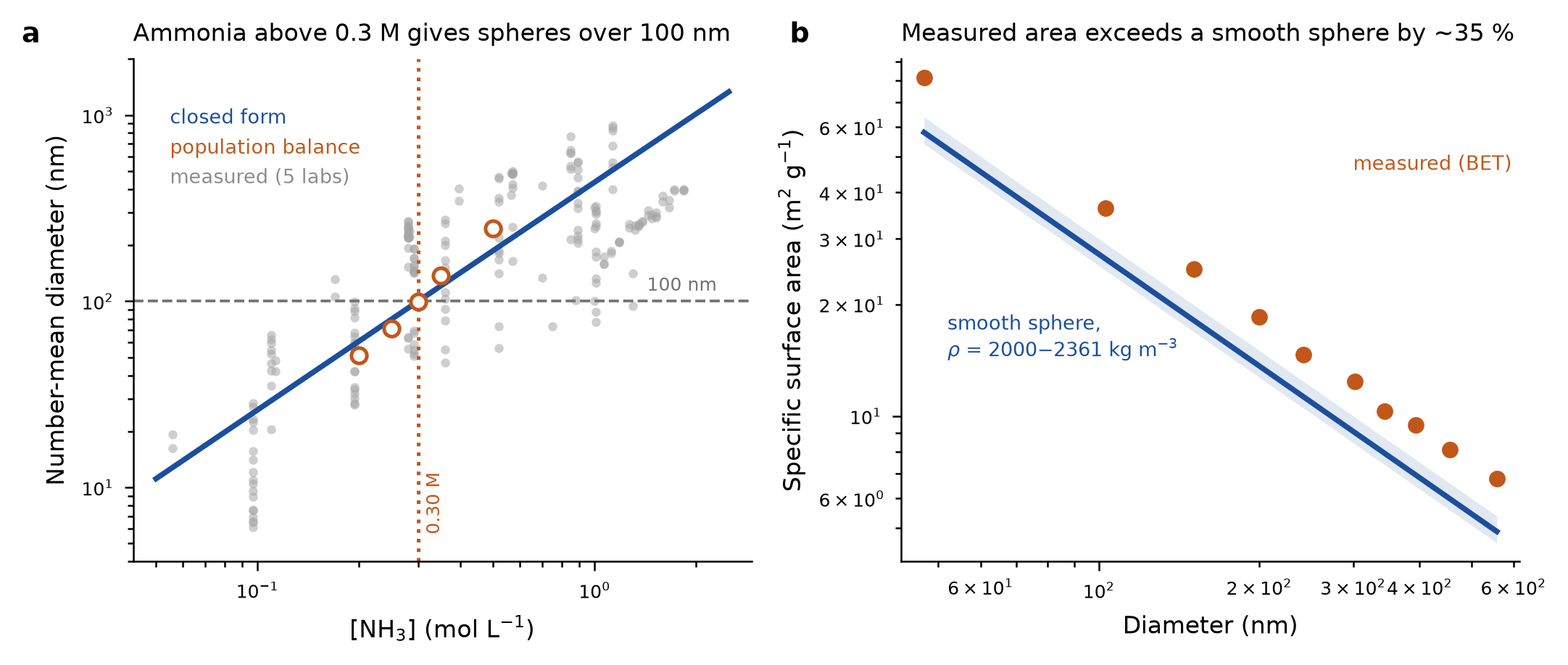
The produced figure: the conditional size crossover and surface-area inference. Saved output from this investigation; no new calculation runs in this page.
Model and method
Yes. Laplace coupled Cantera hydrolysis kinetics to a population-balance model of particle formation and aggregation, then implemented an OpenFOAM comparison. The CFD check covers the first 10 seconds of aggregation. It is numerical verification of a shared model, rather than validation of the complete physical synthesis.
How the investigation developed.
An R&D team wants reproducible silica spheres of a chosen size, using TEOS, ammonia, water and ethanol. It needs a useful process lever and an explanation of what sets the final diameter. Later, the user asks specifically for particles above 100 nm and an estimate of their surface roughness. The practical decision is which synthesis condition to vary next and what to measure alongside it.
01
Build the process model and keep its bookkeeping honest
Laplace assembled a reusable simulation package, parameter provenance, tests and figures. It coupled hydrolysis kinetics to an aggregation-based particle population balance, with silicon conservation as a numerical check. A second implementation in OpenFOAM reproduced the mean diameter to about 0.012% at the 10-second endpoint on the same size grid. That supports implementation consistency; two solvers can still share an incorrect physical model.
02
Find out why a plausible model misses the observations
A fixed literature stability parameter produced only a narrow band of diameters, while the assembled measurements spanned much more. Laplace derived how the stability barrier controls the point where aggregation stops, fitted its dependence on conditions, and tested transfer by leaving out one publication at a time. The fit’s 40% median error became 57–178% on held-out publications. That changes the handoff: a fitted literature correlation is not a laboratory-ready recipe.
03
Translate the model into the next synthesis test
For a specified scenario of 0.28 M TEOS, 6 M water, 25 °C and two hours, the fitted model places the 100 nm diameter crossover near 0.30 M ammonia. The recorded population-balance run gives 99.4 nm at that condition. Within this scenario, ammonia is a useful variable to test. A later roughness estimate came from published surface-area measurements, not from the particle-size simulation, which tracks spherical volumes and cannot predict surface texture.
Two implementations, one clearly bounded checkOriginal result
Original session figure. Batch and OpenFOAM trajectories are compared on matched and different size grids. The 0.012% endpoint agreement belongs to an identical 21-section grid over the first 10 seconds; the result verifies implementation consistency, not material prediction accuracy. cfd_vs_wellmixed_2.png · Evidence summary ↗
Make the prediction error visibleOriginal result
Original session figure for the fitted dataset, coloured by publication. The final fit has about 40% median relative error. Held-out-publication errors of 57–178% are not displayed in this parity chart and are reported separately in cross_validation.csv. fig_parity.png · Evidence summary ↗
A conditional process lever, and a different source for roughnessOriginal result
Original later-session artifact. Left: fitted and simulated size versus ammonia under stated conditions. Right: literature BET area compared with a smooth-sphere calculation. The right panel is a measurement-based inference with porosity and density assumptions, not a simulated external roughness prediction. fig_size_roughness.png
The next test
Run a controlled synthesis series in one laboratory, varying ammonia and measuring both time-resolved size and particle number. Those observations can separate kinetics from aggregation effects and test whether the literature-derived crossover transfers. Characterise porosity and external texture separately before using the surface-area estimate as roughness.
Scientific assumptions and limitations
The 0.012% number is agreement between implementations at one 10-second endpoint. It is not experimental accuracy, whole-run agreement or validation of the final arrest size.
The 40% median error is in-sample. Held-out-publication median errors range from 57% to 178%; the fitted recipe hypothesis needs controlled local validation.
The nominal 0.30 M ammonia crossover applies to a fitted scenario with fixed TEOS, water, temperature and time. It is not a validated production recipe or a general threshold.
Distribution widths do not converge with the size grid and remain upper bounds. Some reaction coefficients have no source; condensation is disabled and the unsupported classical-nucleation route does not run.
Surface roughness was inferred from one publication’s BET surface-area data and assumed density; internal porosity and external texture are confounded. No atomistic roughness simulation or ReaxFF trajectory was completed.
The separate sodium-silicate/sulfate export shares a project ID but has cancelled status and zero artifacts. Its promised workflow is not a completed result and does not establish sulfate effects for this TEOS-based case.
The same questionWhich synthesis condition should we vary to target larger silica spheres?
Direct the investigation. Inspect the work.
Laplace carries technical execution while researchers set the question, steer the study, and evaluate the evidence.
A team-managed workflowIllustrative workflow with existing tools
Task 1Reconcile recipes and sources
→
Task 2Implement the coupled model
→
Task 3Fit and cross-check
→
Task 4Explore process conditions
→
Task 5Design the next experiment
The team coordinates tools, context, and revisions across the study.
With LaplaceTechnical work demonstrated in these studies
HUMANBrief + steer
Laplace carries the technical work
Assemble the source datasetBuild an executable process modelTest implementation and transferIdentify a conditional process leverDeliver code, limits and a test plan
↺ Run → inspect → revise, with researcher steering
HUMANReview + decide
Task execution delegatedModel setup, code and output processing are carried inside the recorded investigation.
Revisions stay connectedChanges to the brief and diagnostic corrections share a working record.
Results arrive togetherInspect the files, findings and next test in one handoff.
Illustrates work ownership. Box widths are schematic; human time saved was not measured.
Inspect the work inside the Laplace block
Assemble the source dataset. Record 209 published measurements and parameter provenance.
Build an executable process model. Couple Cantera kinetics to particle aggregation and silicon balance.
Test implementation and transfer. Compare OpenFOAM on a matched grid; hold publications out of fitting.
Identify a conditional process lever. Explore ammonia dependence and a scenario near 100 nm.
Deliver code, limits and a test plan. Keep roughness inference separate; specify controlled time-series data.
↺Numerical checks and held-out errors determine whether to revise the model or collect better data.
Data reconciliation, modelling, fitting and verification become one connected investigation. Solver agreement and physical prediction error remain separate evidence.
What this study gathered.
Evidence gathered
209 literature rows + solver checks
Five publications, 207 fitted rows, OpenFOAM comparisons and process scans.
A conventional route would collect recipes and kinetic data, resolve concentration and unit conventions, choose a growth mechanism, implement particle-number and mass balances, fit uncertain parameters, and compare with experiments. A CFD specialist could then check whether spatial transport changes the well-mixed calculation. This is model-building and data reconciliation as much as it is running a solver. No matched expert-effort baseline was recorded.
How to read the timing
These investigations often continued across separate visits. The first and last messages do not measure continuous work.
2d 04h 09m 19sCalendar span of the conversation
3h 36mCombined child-agent windows, with overlapping intervals counted once
Agent windows can include waiting and omit work in the main conversation. They are not a measure of active human work, total compute or time saved. The exports do not provide a reliable labour clock.
create a model for fludiztion of silica 500 nm spheres powder; search for relevant open source programcreate a model for fludiztion of silica 500 nm spheres powder; search for relevant open source programcreate a model for fludiztion of silica 500 nm spheres powder; search for relevant open source program
Research prompt↑
LLaplaceRecorded result
Clumps, vibration, and the next experiment.
A 1,600-clump particle study explored vibration. A separate analytical model estimated a conditional gas-velocity range; the particle runs themselves contained no gas.
The particle runs contain no gas and their initial packing was still settling. Clump size is calibrated; this is not a validated fluidized-bed operating point.
Force estimates, particle simulations and numerical review expose which parts of a powder-flow explanation survive scrutiny.
The particle simulation contains no gas, and its control bed was still settling. It does not yet establish a vibration-driven fluidization effect.
The powder problem changes when you model the clumps.
Very fine powder behaves as collections of clumps rather than isolated primary particles. Laplace modelled the clumps, explored a conditional gas-velocity range, and simulated vibration in a small particle system. The work identified clump characterisation and a stable control as prerequisites for testing a useful operating condition.
Study scope. The particle runs contain no gas and their initial packing was still settling. Clump size is calibrated; this is not a validated fluidized-bed operating point.
Inspect the result evidence and download the outputs
A conditional operating estimate: The calibrated model gives fluidization onset near 53.7 mm/s, assuming 250 µm clumps. Evidence ↗
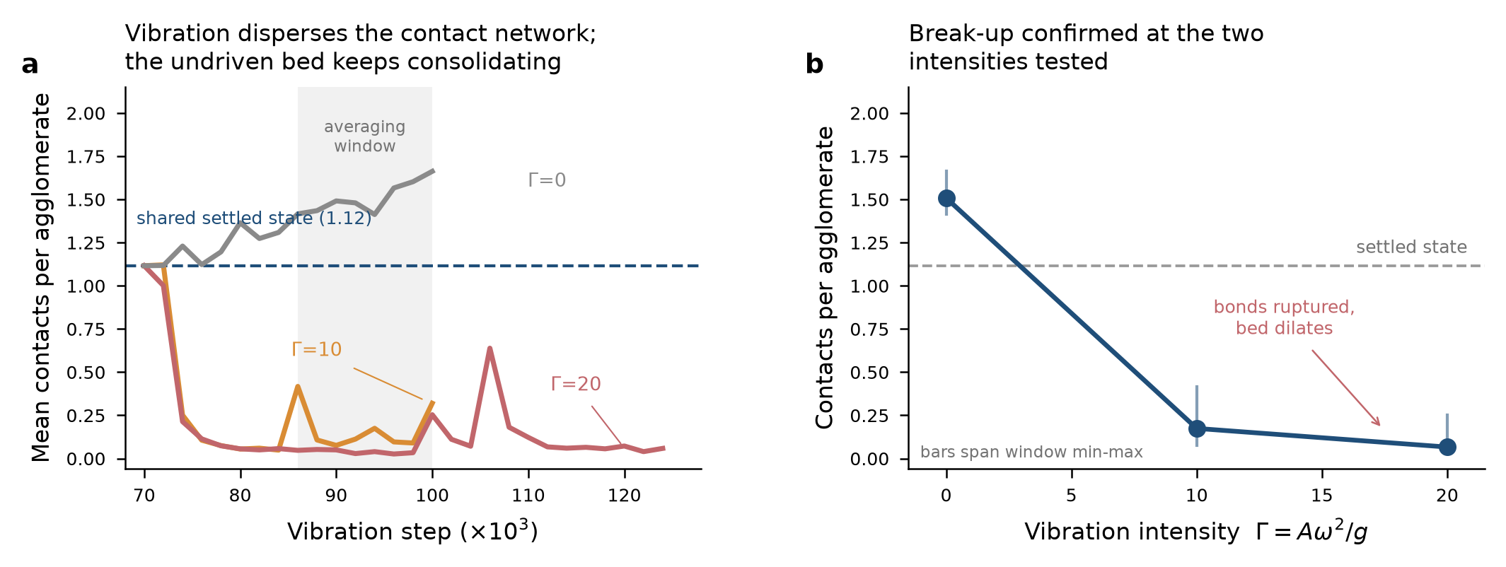
A recorded particle-simulation result: Mean contacts fall from 1.508 without vibration to 0.0666 at Γ = 20 in the shared analysis window. Evidence ↗
An inspectable handoff: A 32-page report, input decks, data and an 82-row ledger, alongside reproduction and referee reports. Evidence summary ↗
No gas was simulated in the particle runs and no CFD deck was executed. The clump size is calibrated, the comparison baseline is still settling, and no experiment validates the operating estimate. The chart’s stronger “network” wording is qualified by the report’s own limitations.
1,600Clumps in the particle simulationA small periodic patch at three vibration intensities. No gas phase or full vessel simulation.Evidence summary ↗
1.51 → 0.067Mean contacts per simulated clumpWithout vibration versus Γ = 20, in the same eight-sample window. The starting state was still settling.Source ↗
53.7 mm/sModelled onset of fluidizationConditional on a calibrated 250 µm clump size. Not a measured operating setpoint.Source ↗
The produced figure: contact counts under three vibration conditions. Saved output from this investigation; no new calculation runs in this page.
Model and method
Yes. Laplace ran an algebraic agglomerate model, a 400-point gas-velocity sweep and LAMMPS discrete-element simulations of 1,600 agglomerates under vibration. The particle simulations contain no gas. MFiX and LIGGGHTS input decks were produced but never executed, so this session does not demonstrate a completed CFD fluidization study.
How the investigation developed.
A team wants to handle a powder made of 500 nm silica spheres. Blowing gas through a powder bed can help expose the material for drying, coating or reaction, but these tiny particles stick together. The useful question is what the gas would actually move, which conditions could mobilise it, and whether vibration is worth testing. These are proposed industrial applications, not evidence of an existing customer deployment.
01
Model the clump that the gas must move
Under the stated dry-contact assumptions, adhesion between primary particles is about six million times a particle’s weight. Laplace therefore represented a hierarchy of clumps rather than treating every 500 nm sphere as freely dispersed. A fitted constant sets the larger clump diameter to 250 µm. Given that calibration, the model estimates fluidization onset near 53.7 mm/s and terminal velocity near 410 mm/s. The size is a calibration input, so the apparent operating window is a hypothesis to test.
02
Test contact separation with a second kind of model
Laplace ran a LAMMPS study of 1,600 clumps, comparing no vibration with two imposed vibration intensities. In archived repeat-run traces, mean contact counts over the common window fall from 1.508 to 0.174 and 0.0666. This supports a vibration-dependent contact-separation trend in the simulated system. The calculation contains no gas and does not measure process throughput, coating quality or complete fluidization.
03
Use review to expose the assumption that controls the answer
The export contains a separate reproduction audit, a referee report and subsequent corrections. They expose missing model definitions, inconsistent numbers and a baseline that was still settling. The final report acknowledges that contact softening changes the physical contact regime and that the clump size is calibrated. Repeated simulation averages differ from the original run averages by 17–48% over different windows. The useful handoff is a model and a measurement plan with explicit limits, rather than a production setting.
The model starts with the clumps, not just the primary particlesOriginal result
Original multi-panel model figure. The 250 µm clump size is calibrated; the operating range and sensitivity curves depend on the stated assumptions. The proposed roughness, vibration and pressure-drop signatures are model outputs, not measured process improvements. fluidization_model.png · Evidence summary ↗
A conditional gas-velocity sweepOriginal result
Original session figure from the algebraic model’s 400-point sweep. Despite “TFM” in the filename, this is not an executed MFiX CFD calculation. The fluidization onset and expansion curves inherit the calibrated clump size. step1_tfm_sweep.png · Evidence summary ↗
Vibration reduces contacts in the simulated particle assemblyOriginal result
Original LAMMPS figure. Common-window means are 1.508, 0.174 and 0.0666 contacts at Γ = 0, 10 and 20. Γ denotes vibration acceleration relative to gravity. The source artwork says “network” and “break-up confirmed”; the final limitations describe a sparse assembly with a drifting baseline. This is contact separation in a gas-free simulation, not validated fluidization or internal clump fragmentation. step2_dem_breakup.png · Evidence summary ↗
The next test
Measure the real powder’s clump size and pressure drop as gas velocity changes, while recording humidity. For a stronger vibration test, first settle the simulated packing to a stable baseline and examine contact-model and domain sensitivity. Then use coupled gas–solid simulation or a controlled bench test to check the proposed operating range.
Scientific assumptions and limitations
The 250 µm agglomerate diameter is a calibration target, not an independent prediction. The 53.7 mm/s onset and roughly 410 mm/s terminal velocity inherit that assumption. No experimental validation of this powder was performed.
The LAMMPS runs contain no gas. They track contacts between rigid model agglomerates, not the internal fragmentation of 500 nm primary-particle clusters or a complete fluidized bed. MFiX and LIGGGHTS decks were generated but not executed or syntax-verified.
The shared initial packing was still settling. Each vibration condition used one deterministic realisation in a small periodic box, with eight samples in the quoted window. The comparison does not isolate vibration from all initial-state effects or establish an industrial benefit.
Contacts were softened from 70 GPa to 10 MPa for tractable time steps. The final report acknowledges a change in contact regime; preserving the chosen pull-off force does not validate the physical contact response.
Original and repeated runs use different averaging windows; reported means differ by 17–48%. The record supports the trend and its scale, not precise reproducibility of every value.
The archived audit and referee report concern an earlier draft. The final PDF incorporates corrections but retains inconsistent wording, including stronger network claims than its own sparse-packing limitation supports. The reproduced continuum table is not a clean audit pass of the entire final document.
No measured human-hours saving, complete billing comparison, production throughput improvement or customer outcome is established. The recorded session span includes unknown waiting, compute and human interaction.
The same questionWhat moves when gas passes through fine silica powder, and is vibration worth testing?
Direct the investigation. Inspect the work.
Laplace carries technical execution while researchers set the question, steer the study, and evaluate the evidence.
A team-managed workflowIllustrative workflow with existing tools
Task 1Characterise the powder
→
Task 2Choose models and solvers
→
Task 3Build and run calculations
→
Task 4Reproduce and challenge
→
Task 5Prepare the bench study
The team coordinates tools, context, and revisions across the study.
With LaplaceTechnical work demonstrated in these studies
HUMANBrief + steer
Laplace carries the technical work
Identify the relevant particle scaleAssemble the process modelRun a bounded particle studyAudit the numerical storyDeliver a testable handoff
↺ Run → inspect → revise, with researcher steering
HUMANReview + decide
Task execution delegatedModel setup, code and output processing are carried inside the recorded investigation.
Revisions stay connectedChanges to the brief and diagnostic corrections share a working record.
Results arrive togetherInspect the files, findings and next test in one handoff.
Illustrates work ownership. Box widths are schematic; human time saved was not measured.
Inspect the work inside the Laplace block
Identify the relevant particle scale. Represent larger clumps; set a 250 µm calibration target.
Assemble the process model. Calculate conditional gas-flow and bed-expansion behaviour.
Run a bounded particle study. Simulate 1,600 clumps at three vibration intensities, without gas.
Audit the numerical story. Archive repeat traces, a reproduction audit and reviewer corrections.
Deliver a testable handoff. Provide the report, data, code and the missing physical checks.
↺The audit sends the study back to clump-size calibration, a stable baseline and the right contact physics.
Solver selection, model formulation, execution and critical review become one documented investigation. The unresolved physical assumptions determine the next experiment.
What this study gathered.
Evidence gathered
400 sweep points + particle traces
Three vibration conditions, input decks, 82-row ledger and a 32-page report.
A conventional investigation would combine powder characterisation, cohesion and drag models, solver selection, particle-contact simulations and bench measurements. Specialists would decide which particle scale to represent, transfer parameters between models, check numerical sensitivity and write a report that distinguishes computed trends from experimentally established settings. No matched conventional project or active-effort log was supplied.
How to read the timing
These investigations often continued across separate visits. The first and last messages do not measure continuous work.
2d 18h 51m 42sCalendar span of the conversation
4h 17mCombined child-agent windows, with overlapping intervals counted once
Agent windows can include waiting and omit work in the main conversation. They are not a measure of active human work, total compute or time saved. The exports do not provide a reliable labour clock.
Use FDS to predict a vegetation fire on sloped terrain.Use FDS to predict a vegetation fire on sloped terrain.Use FDS to predict a vegetation fire on sloped terrain.
Research prompt↑
LLaplaceRecorded result
Four slopes. Temperature and flow made visible.
FDS runs at 0°, 10°, 20°, and 30° produced fields, diagnostics, and comparison movies to investigate how terrain changes the fire.
Reference grass fuel and no wind. Steep scenarios also use longer fuel beds and shorter ignition; slope is not isolated alone. Absolute spread rates remain unvalidated.
Parallel fire simulations connect the case setup to flame fields, spread measurements and movies.
Reported solver time per run, excluding setup and analysis. The steeper cases use a longer fuel bed and shorter ignition, so this is not a controlled slope-only comparison.
Watch the result Original session films
Four slopes on one simulation clock8.5s playback
Original landscape MP4, identified in the final response as rebuilt after the mesh-slice correction. The on-screen time is simulated time. Geometry, fuel and validation limits are described below.
Playback length is separate from simulated time and the session span.
Four slopes turn a fire question into a visible mechanism.
A slope changes the geometry between a fire, its hot gases, and the fuel ahead. Laplace configured and ran FDS cases at 0°, 10°, 20°, and 30°, inspected ignition effects, and produced temperature fields, flow fields, and movies. Explore the recorded results to examine the proposed slope-attachment mechanism.
Study scope. Reference grass fuel and no wind. Steep scenarios also use longer fuel beds and shorter ignition; slope is not isolated alone. Absolute spread rates remain unvalidated.
Inspect the result evidence and download the outputs
Computed scenario results: Final spread rates: no sustained propagation at 0°, then 1.79, 58.72 and 138.71 cm/s at 10°, 20° and 30°. Evidence ↗
Visible physical mechanism: The computed plume changes from upright to nearly aligned with the fuel surface in the steeper cases. Evidence ↗
Original shareable output: Landscape and portrait MP4s produced from the corrected fields, alongside the 12-page report and input decks. Evidence ↗
The movies show recorded simulation outputs, not footage of real fires. This study uses reference fuel, zero wind and one grid resolution. The steep cases remain domain-limited, and there is no experimental validation or measured labour-saving comparison.
4 slopesCompleted research scenarios0°, 10°, 20° and 30°, using the same reference grass properties. Steep cases needed longer beds and shorter ignition.Source ↗
1.79 → 138.71Modelled spread rate, cm/s: 10° to 30°Scenario outputs, not field measurements. Reported fit errors exclude grid, fuel and model uncertainty.Source ↗
Explore recorded results · 4 FDS scenarios
Change the slope. Inspect the flame.
Switch between the original simulated temperature and flow fields. Watch how the plume lies closer to the fuel in the steeper cases.
Display a field
Gas temperature and the 300 °C flame contour
A viewport into the unchanged original figure. Coordinates follow the model’s slope-aligned frame. The selected snapshots are from different model times, not a synchronized animation.
Recorded spread rate1.79 cm/sFit after the igniter was switched off
Reported mean flame tilt19.2°Across the source’s sampled frames
Reference fuel and zero wind. Steep cases use a longer fuel bed and earlier igniter cutoff; this is not a perfectly isolated single-parameter experiment. Absolute spread rates are unvalidated and the steep cases remain limited by domain size.
Model and method
Yes. The session records execution of Fire Dynamics Simulator on the the compute environment cluster, coupling a reacting surface fuel bed with gas flow, combustion and radiation. The final comparison covers 0°, 10°, 20° and 30° slopes with zero ambient wind. This is an idealised line-fire research study on a single grid resolution, with no validation against physical fire measurements.
How the investigation developed.
A researcher wants to understand how terrain slope changes a vegetation fire. The prompt specifies FDS and an available compute cluster, but leaves the geometry, fuel representation, scenario design and analysis to the investigation. The practical research decision is which mechanism and conditions merit more detailed simulation or a controlled burn experiment.
01
Turn a slope question into runnable physical scenarios
Laplace represented a planar slope by rotating gravity while keeping the fuel bed aligned with the computational grid. It used reference dry-grass properties, zero ambient wind and a 31.25 mm cell size. The final input decks contain 196,608 cells for shallow slopes and 491,520 for the longer steep-slope cases. The session also caught a cluster-launch problem: some launch commands exited successfully while FDS reported only one process. It checked the reported rank counts before proceeding.
02
Reject a plausible number when it answers the wrong question
In the first steep-slope runs, the entire 3 m fuel bed ignited before the ignition source switched off. A tidy line fit could still be made, but it described the ignition setup rather than a front continuing on its own. Laplace reran 20° and 30° on 9 m beds with a shorter ignition period and fitted only arrivals after the igniter stopped. The final table reports no sustained propagation at 0°, then 1.79, 58.72 and 138.71 cm/s at increasing slopes. These remain configuration-dependent predictions.
03
Show the mechanism, then check the visualisation itself
The resolved fields show an upright plume in the shallow cases and a flame lying closer to the fuel in the steep cases. A later request turned those fields into still images and landscape and portrait movies. Review found cold stripes introduced when neighbouring mesh slices were joined incorrectly, plus temperature peaks calculated from reduced-resolution data. The final response records corrections to the assembly code, full-resolution peak diagnostics and rebuilt MP4s. The supplied source movies and revised stills are featured here; this review has not reconstructed their raw fields.
The final scenario comparisonOriginal result
Original result figure after the longer-bed reruns. Rates are model outputs for the stated reference fuel and zero-wind setup. Error bars measure fit precision only. The 20° and 30° cases use different bed length and ignition duration from the shallow cases; grid and experimental validation remain absent. fds_ros_vs_slope.png · Evidence summary ↗
See the plume move toward the fuelOriginal result
Original field visualisation, identified as corrected in the final session response. Each row shows its own selected time and spatial window, so these stills are not a common-time race. Colours show gas temperature and upslope flow; the video above supplies a shared-clock view. fds_flame_structure.png
Connect the pictures to measurable diagnosticsOriginal result
Corrected source figure summarising flame tilt, flow and temperature histories. The diagnostics CSV reports mean tilt from 7.0° to 85.4° and full-field temperature maxima from 1,344.2 to 1,740.3 °C across the scenarios. Tilt variation and front-fit errors are not predictive uncertainty intervals. fds_mechanism.png
Why the first steep-slope setup was rejectedOriginal result
Diagnostic of the initial short-bed runs, retained to explain the correction. All steep-slope probes were heated while the igniter was active. Its steep-slope curves are superseded and must not be used as the final spread-rate result. fds_slope_summary.png · Evidence summary ↗
The next test
Test sensitivity to grid size and fuel-bed length, then reproduce a controlled experiment with measured fuel properties. Only after that evidence should the model be extended to wind, realistic terrain or decisions that require predictive accuracy. The current study helps choose that next research step.
Scientific assumptions and limitations
The fuel is an FDS reference grass set, with 8% moisture and no ambient wind. The geometry is a planar slope and an idealised narrow line-fire configuration with mirror side boundaries. This is not a site-specific wildfire or incident forecast.
Only one grid resolution, 31.25 mm, was tested. No quantitative comparison with a physical fire experiment was performed. Absolute spread rates and the apparent transition between 10° and 20° remain unvalidated scenario results.
The 0° and 10° cases use 3 m beds and 16-second ignition; 20° and 30° use 9 m beds and 8-second ignition. The change addresses ignition contamination, but the final matrix is not identical in all settings except slope. The steep cases remain domain-limited and accelerating.
The ± values in the source table are standard errors of a fitted line, not total prediction uncertainty. A high fit score does not validate the model or remove ignition, fuel and resolution effects.
The final MP4s and two field figures are identified in the session as corrected versions. Earlier GIFs predate the slice-assembly fix and are preserved in the archive rather than featured as corrected results.
The supplied ZIP omits raw device histories, raw field files and corrected field arrays. Input decks and summaries can be inspected, but the spread fits, field reconstruction and claimed checksum checks cannot be independently reproduced from the supplied bundle alone.
The technical-memorandum styling follows the user’s report-format request; it does not establish NASA or NIST authorship, review or endorsement of this study. Reported cluster runtime and core-hours do not establish total cost or human time saved.
A conventional study would ask a fire modeller to define the fuel and geometry, configure a parallel solver, run a slope matrix, diagnose ignition and domain effects, extract front trajectories and turn large field outputs into reports and visualisations. Model setup, cluster execution, scientific interpretation and communication are distinct pieces of work that must remain consistent. No matched specialist-effort baseline was supplied.
How to read the timing
These investigations often continued across separate visits. The first and last messages do not measure continuous work.
08h 06m 36sCalendar span of the conversation
54mCombined child-agent windows, with overlapping intervals counted once
Agent windows can include waiting and omit work in the main conversation. They are not a measure of active human work, total compute or time saved. The exports do not provide a reliable labour clock.
create a sample WRF weather simulationcreate a sample WRF weather simulationcreate a sample WRF weather simulation
Research prompt↑
LLaplaceRecorded result
A simulated storm. A simpler explanation to compare.
Two simulated hours in WRF became a storm-splitting investigation, followed by a reduced physical model and a paper comparing selected diagnostics.
One idealized WRF atmosphere, not a real-world forecast. Agreement varies by diagnostic; the source paper retains rainfall-window and vorticity-caption inconsistencies.
A parallel weather model supplies the storm fields; automated analysis connects them to a simpler model and its limits.
Grid points are calculated from the recorded 80 × 80 × 40 grid. Two hours describes simulated weather, not compute time. The simpler model was tuned after the reference run.
A working storm simulation becomes an explanation to test.
A short request for a weather simulation grew into an investigation of storm splitting. Laplace ran an idealized WRF case, developed a reduced physical model, and compared selected outputs. The differences show which mechanisms the simpler model captures and which need further testing.
Study scope. One idealized WRF atmosphere, not a real-world forecast. Agreement varies by diagnostic; the source paper retains rainfall-window and vorticity-caption inconsistencies.
Inspect the result evidence and download the outputs
Executed virtual experiment: Two hours of idealized storm evolution with nine diagnostic snapshots and two tracked storm cores. Evidence ↗
Testable explanation: The reduced model gives a 39.8 m/s peak updraft against 44.9 m/s in the mature WRF profile; removing rotation lowers it to 34.6 m/s. Evidence ↗
Produced research artifact: An eight-page article, three original figures, configuration files and saved numerical outputs. Evidence summary ↗
This is a single idealized model-to-model study. The paper retains unequal rainfall time windows and stronger accuracy language than the evidence supports. It does not establish real-weather forecast accuracy or measured time savings.
2 hoursWeather evolution simulatedNine diagnostic snapshots, every 15 minutes. This is simulated time, not compute time or a real forecast.Source ↗
39.8 vs 44.9Peak updraft, simplified model vs WRF · m/s11.3% lower in the simplified model. WRF value is the peak of the mature-phase mean profile, not the single largest instantaneous updraft.Source ↗
The produced storm maps and evolution chart. Saved output from this investigation; no new calculation runs in this page.
Model and method
Yes. The session records building and running WRF-ARW 4.6.1 on 16 MPI ranks for an idealized supercell: a rotating thunderstorm. It simulates two hours on an 80 × 80 × 40 grid with 2 km horizontal spacing. A second, numerically integrated plume model uses the same initial atmospheric profile to explain selected outputs. No real weather observations initialize or validate this study.
How the investigation developed.
A research team wants a working storm example and a physical explanation of its behaviour. A colourful map can show a storm splitting, but it does not explain which assumptions control its strength, motion or rainfall. The useful next decision is which features a simple model can represent and which need fuller three-dimensional dynamics.
01
Turn six words into a working virtual experiment
The initial request was “create a sample WRF weather simulation”. Laplace selected WRF’s existing quarter-circle-shear supercell test, repaired a source-build dependency problem and ran the model on the available cluster. A warm bubble in a prescribed atmosphere develops into two storm cores with opposite rotation. The diagnostic series reaches a peak instantaneous updraft of 46.9 m/s at 45 minutes and a maximum accumulated rainfall of 64.5 mm at two simulated hours. These are outputs of the idealized case, not observed weather.
02
Ask the simulation a second question: why?
The user then requested an analytical first-principles explanation and a paper. Laplace assembled a reduced plume model using the initial temperature, moisture and wind profile, with assumptions for mixing, water loading and rotation. It produced a 39.8 m/s peak updraft against 44.9 m/s in the mature WRF profile. Removing the rotational contribution lowers the reduced-model result to 34.6 m/s. That creates a testable explanation within the model: quantify what a mechanism changes, then compare it with the richer simulation.
03
Keep the mismatches in the story
The simpler model comes close to the right-moving storm’s speed, but overestimates the left-moving speed by about 46% and peak vorticity by about 53%. Its storm-area growth is about 62% too low. Review corrected the reported rotation ranges and the storm figure. A rainfall table still compares a 90-minute model accumulation with a two-hour WRF total. The result is a useful research package with visible unresolved questions; the manuscript’s broad accuracy language goes beyond what this one case establishes.
One storm becomes two: the produced simulationOriginal result
Original WRF figure. Read left to right through 30, 60, 90 and 120 simulated minutes. Colours show a computed radar-like signal; markers track two storm cores moving apart. The lower panels show a vertical slice and the time history of rising-air speed and storm area. This is a virtual atmosphere, not radar observations. wrf_supercell_evolution.png
From a complex output to a physical explanationOriginal result
Original analytical-model figure. In the lower-left panel, the solid blue updraft profile is compared with the black WRF profile; the dashed blue curve removes rotation from the reduced model. Supplied arrays confirm peaks of 39.8, 44.9 and 34.6 m/s respectively. This checks the plotted comparison, not the validity of the physical closure. fig_model.png · Evidence summary ↗
Make the differences visible alongside the agreementsOriginal result
Original comparison figure, preserved unchanged. The reduced model is sensitive to its assumed radius, and some predicted quantities differ substantially from WRF. The rain point uses unequal accumulation windows; the vorticity profile peaks near 9 km despite a manuscript caption claiming a 2–5 km peak. Treat this as a diagnostic figure, not proof of general forecasting accuracy. fig_verification.png · Evidence summary ↗
The next test
Reconcile the rainfall time windows and diagnostic definitions, check the sensitivity to assumed plume radius and WRF grid spacing, then test the reduced model on new atmospheric profiles. Keep a held-out benchmark and measured specialist effort so a future study can establish transfer and time saved.
Scientific assumptions and limitations
This uses WRF’s existing idealized supercell test, initialized from an analytic atmospheric profile and a warm bubble. It is not a new forecasting engine or a forecast for a place and date. The setup omits radiation, surface and boundary-layer schemes.
Only one atmospheric profile and one 2 km grid were studied. The reference is another simulation, not measured weather. Agreement with WRF cannot establish real-world accuracy or performance on new storms.
The reduced model uses a chosen radius closure R = H/π and other physical assumptions. The source says no parameter was tuned to WRF, but the model was developed after the WRF output was available. This is not a blind held-out prediction or proof of a universally valid first-principles derivation.
The paper’s 11% median discrepancy must not become a blanket accuracy claim. Selected quantities differ substantially: left-moving speed by about +46%, peak vorticity by +53% and echo-area growth by −62%. The plotted comparisons and prose summaries use different selections of quantities.
The rainfall row labelled “Peak accumulation (2 h)” uses approximately 42 mm from a 27.9 mm/h model rate multiplied by 1.5 hours, versus 64.5 mm after two WRF hours. The source reviewer flagged this and the supplied final manuscript retains it. Its −35% figure is not a comparison over equal durations.
The reduced-model vorticity profile peaks near 9 km in the supplied arrays. The manuscript caption says its peak matches the 2–5 km layer; that wording is not supported by the supplied profile. The claimed grid-resolution explanation for vorticity disagreement also lacks a finer-grid test.
The ZIP supplies 12 files for 21 artifact records: eight earlier WRF fields and paper_build.tex are absent. It contains the final WRF field and reduced-model arrays, but no standalone model integration script. The original TeX retains FIGMODEL/FIGVERIF placeholders. This is an inspectable archive, not a complete independently reproduced study.
The eight-page PDF follows the user’s requested article format; no arXiv publication or independent peer review is established. Session review corrected some issues but did not resolve every scientific or presentation claim. The roughly 90-second solver runtime stated in the paper excludes installation, analysis, writing and review.
A specialist would install and configure a weather model, choose an idealized test, run it on available compute, extract storm tracks and profiles, formulate a simpler model, compare like quantities and write up the findings. That combines software setup, numerical modelling, atmospheric physics and communication. The supplied record has no matched conventional project or measured expert hours.
How to read the timing
These investigations often continued across separate visits. The first and last messages do not measure continuous work.
03h 20m 25sCalendar span of the conversation
29mCombined child-agent windows, with overlapping intervals counted once
Agent windows can include waiting and omit work in the main conversation. They are not a measure of active human work, total compute or time saved. The exports do not provide a reliable labour clock.
Each study connects its physical question to the recorded result, model assumptions and selected scientific files.
Numerical results with their limits
Synthetic observations, reduced models and comparisons between solvers are identified in the study. Numerical agreement does not by itself establish physical validation.
A focused technical handoff
Explore selected tables, figures, movies and scientific Python scripts. The public evidence summaries are curated explanations. Some original inputs and dependencies are unavailable, so the downloads are not complete reproducibility packages.